Handling multi-dimensional arrays with xarray
Contents
Handling multi-dimensional arrays with xarray#
Context#
We will be using the Pangeo open-source software stack for computing and visualizing the Vegetation Condition Index (VCI) [Kog95], a well-established indicator to estimate droughts from remote sensing data.
VCI compares the current normalized difference vegetation index (NDVI) [Wik2)] to the range of values observed in previous years.
Data#
In this episode, we will use Sentinel-3 NDVI Analysis Ready Data (ARD) provided by the Copernicus Global Land Service.
This dataset can be discovered through the OpenEO API from the CGLS distributor, VITO. Access is free of charge but an EGI registration is needed.
The same dataset can also be downloaded from Zenodo: FOSS4G Training Datasets: NDVI
Further info about drought indices can be found in the Integrated Drought Management Programme (see here).
Setup#
This episode uses the following main Python packages:
Please install these packages if they are not already available in your Python environment (see Setup page).
Packages#
In this episode, Python packages are imported when we start to use them. However, for best software practices, we recommend that you install and import all the necessary libraries at the top of your Jupyter notebook.
import xarray as xr
Fetch Data#
For now we will fetch a netCDF file containing Sentinel-3 NDVI Analysis Ready Data (ARD).
The file is available in a Zenodo repository. We will download it using using
pooch, a very handy Python-based library to download and cache your data files locally (see further info here)In the Data access and discovery episode, we will learn about different ways to access data, including access to remote data.
import pooch
cgls_file = pooch.retrieve(
    url="https://zenodo.org/record/6969999/files/C_GLS_NDVI_20220101_20220701_Lombardia_S3_2.nc",
    known_hash="md5:bbb25f1865056c886c6f9b37147d8f2f",
    path=f".",
)
Downloading data from 'https://zenodo.org/record/6969999/files/C_GLS_NDVI_20220101_20220701_Lombardia_S3_2.nc' to file '/home/runner/work/foss4g-2022/foss4g-2022/tutorial/pangeo101/4d4b4841cc038396b6f78fb014a6b538-C_GLS_NDVI_20220101_20220701_Lombardia_S3_2.nc'.
Open and read metadata through Xarray#
cgls_ds = xr.open_dataset(cgls_file)
As the dataset is in the NetCDF format, Xarray automatically selects the correct engine (this happens in the background because engine=’netcdf’ has been automatically specified). Other common options are “h5netcdf” or “zarr”. GeoTiff data can also be read, but to access it requires rioxarray, which will be quickly covered later. Supposing that you have a dataset in an unrecognised format, you can always create your own reader as a subclass of the backend entry point and pass it through the engine parameter.
Tip
If you get an error with the previous command, first check the location of the input file some_hash-C_GLS_NDVI_20220101_20220701_Lombardia_S3_2.nc: it should have been downloaded in the same directory as your Jupyter Notebook.
cgls_ds
<xarray.Dataset>
Dimensions:  (t: 20, x: 984, y: 657)
Coordinates:
  * t        (t) datetime64[ns] 2022-01-01 2022-01-11 ... 2022-07-01 2022-07-11
  * x        (x) float64 8.502 8.505 8.508 8.511 ... 11.42 11.42 11.42 11.43
  * y        (y) float64 46.63 46.63 46.63 46.62 ... 44.69 44.69 44.68 44.68
Data variables:
    crs      |S1 b''
    NDVI     (t, y, x) uint8 ...
Attributes:
    Conventions:  CF-1.8
institution: openEO platformWhat is xarray?#
Xarray introduces labels in the form of dimensions, coordinates and attributes on top of raw NumPy-like multi-dimensional arrays, which allows for a more intuitive, more concise, and less error-prone developer experience.
How is xarray structured?#
Xarray has two core data structures, which build upon and extend the core strengths of NumPy and Pandas libraries. Both data structures are fundamentally N-dimensional:
DataArray is the implementation of a labeled, N-dimensional array. It is an N-D generalization of a Pandas.Series. The name DataArray itself is borrowed from Fernando Perez’s datarray project, which prototyped a similar data structure.
Dataset is a multi-dimensional, in-memory array database. It is a dict-like container of DataArray objects aligned along any number of shared dimensions, and serves a similar purpose in xarray as the pandas.DataFrame.
Accessing Coordinates and Data Variables#
DataArray, within Datasets, can be accessed through:
the dot notation like Dataset.NameofVariable
or using square brackets, like Dataset[‘NameofVariable’] (NameofVariable needs to be a string so use quotes or double quotes)
cgls_ds.t
<xarray.DataArray 't' (t: 20)>
array(['2022-01-01T00:00:00.000000000', '2022-01-11T00:00:00.000000000',
       '2022-01-21T00:00:00.000000000', '2022-02-01T00:00:00.000000000',
       '2022-02-11T00:00:00.000000000', '2022-02-21T00:00:00.000000000',
       '2022-03-01T00:00:00.000000000', '2022-03-11T00:00:00.000000000',
       '2022-03-21T00:00:00.000000000', '2022-04-01T00:00:00.000000000',
       '2022-04-11T00:00:00.000000000', '2022-04-21T00:00:00.000000000',
       '2022-05-01T00:00:00.000000000', '2022-05-11T00:00:00.000000000',
       '2022-05-21T00:00:00.000000000', '2022-06-01T00:00:00.000000000',
       '2022-06-11T00:00:00.000000000', '2022-06-21T00:00:00.000000000',
       '2022-07-01T00:00:00.000000000', '2022-07-11T00:00:00.000000000'],
      dtype='datetime64[ns]')
Coordinates:
* t (t) datetime64[ns] 2022-01-01 2022-01-11 ... 2022-07-01 2022-07-11
Attributes:
standard_name: t
long_name: t
axis: Tcgls_ds.t is a one-dimensional xarray.DataArray with dates of type datetime64[ns]
cgls_ds.NDVI
<xarray.DataArray 'NDVI' (t: 20, y: 657, x: 984)>
[12929760 values with dtype=uint8]
Coordinates:
  * t        (t) datetime64[ns] 2022-01-01 2022-01-11 ... 2022-07-01 2022-07-11
  * x        (x) float64 8.502 8.505 8.508 8.511 ... 11.42 11.42 11.42 11.43
  * y        (y) float64 46.63 46.63 46.63 46.62 ... 44.69 44.69 44.68 44.68
Attributes:
    long_name:     NDVI
    units:
grid_mapping: crscgls_ds.NDVI is a three-dimensional xarray.DataArray with NDVI values of type uint8
cgls_ds['NDVI']
<xarray.DataArray 'NDVI' (t: 20, y: 657, x: 984)>
[12929760 values with dtype=uint8]
Coordinates:
  * t        (t) datetime64[ns] 2022-01-01 2022-01-11 ... 2022-07-01 2022-07-11
  * x        (x) float64 8.502 8.505 8.508 8.511 ... 11.42 11.42 11.42 11.43
  * y        (y) float64 46.63 46.63 46.63 46.62 ... 44.69 44.69 44.68 44.68
Attributes:
    long_name:     NDVI
    units:
grid_mapping: crsSame can be achieved for attributes and a DataArray.attrs will return a dictionary.
cgls_ds['NDVI'].attrs
{'long_name': 'NDVI', 'units': '', 'grid_mapping': 'crs'}
Xarray and Memory usage#
Once a Data Array|Set is opened, xarray loads into memory only the coordinates and all the metadata needed to describe it. The underlying data, the component written into the datastore, are loaded into memory as a NumPy array, only once directly accessed; once in there, it will be kept to avoid re-readings. This brings the fact that it is good practice to have a look to the size of the data before accessing it. A classical mistake is to try loading arrays bigger than the memory with the obvious result of killing a notebook Kernel or Python process. If the dataset does not fit in the available memory, then the only option will be to load it through the chunking; later on, in the tutorial ‘chunking_introduction’, we will introduce this concept.
As the size of the data is not too big here, we can continue without any problem. But let’s first have a look to the actual size and then how it impacts the memory once loaded into it.
import numpy as np
print(f'{np.round(cgls_ds.NDVI.nbytes / 1024**2, 2)} MB') # all the data are automatically loaded into memory as NumpyArray once they are accessed.
12.33 MB
cgls_ds.NDVI.data
array([[[255, 255, 255, ..., 255, 255, 255],
        [255, 255, 255, ..., 255, 255, 255],
        [255, 255, 255, ..., 255, 255, 255],
        ...,
        [ 83, 100,  99, ..., 124, 108, 255],
        [121, 120, 112, ..., 124, 123, 255],
        [113,  93,  93, ...,  81, 120, 255]],

       [[255, 255, 255, ..., 255, 255, 255],
        [255, 255, 255, ..., 255, 255, 255],
        [255, 255, 255, ..., 255, 255, 255],
        ...,
        [138, 128, 124, ..., 141, 136, 255],
        [132, 123, 118, ..., 160, 152, 255],
        [131, 126, 120, ..., 141, 144, 255]],

       [[255, 255, 255, ..., 255, 255, 255],
        [255, 255, 255, ..., 255, 255, 255],
        [255, 255, 255, ..., 255, 255, 255],
        ...,
        [129, 127, 127, ..., 126, 130, 255],
        [126, 119, 121, ..., 132, 133, 255],
        [124, 132, 126, ..., 128, 115, 255]],

       ...,

       [[255, 255, 255, ..., 186, 195, 255],
        [ 50,  50, 255, ..., 181, 185, 255],
        [255, 255, 255, ..., 186, 188, 255],
        ...,
        [141, 141, 155, ..., 126, 141, 255],
        [133, 126, 141, ..., 142, 150, 255],
        [128, 122, 118, ..., 200, 180, 255]],

       [[255, 255, 255, ..., 185, 190, 255],
        [ 31,  31, 255, ..., 191, 197, 255],
        [255, 255, 255, ..., 198, 193, 255],
        ...,
        [155, 160, 171, ...,  87,  94, 255],
        [142, 150, 154, ..., 132, 149, 255],
        [136, 140, 153, ..., 161, 128, 255]],

       [[255, 255, 255, ..., 182, 182, 255],
        [255, 255, 255, ..., 195, 197, 255],
        [255, 255, 255, ..., 194, 197, 255],
        ...,
        [165, 162, 162, ..., 118, 120, 255],
        [166, 153, 152, ..., 157, 157, 255],
        [159, 141, 142, ..., 175, 166, 255]]], dtype=uint8)
Renaming Coordinates and Data Variables#
As other datasets have dimensions named according to the more common triad lat,lon,time a renomination is needed.
cgls_ds = cgls_ds.rename(x='lon', y='lat', t='time')
cgls_ds
<xarray.Dataset>
Dimensions:  (time: 20, lon: 984, lat: 657)
Coordinates:
  * time     (time) datetime64[ns] 2022-01-01 2022-01-11 ... 2022-07-11
  * lon      (lon) float64 8.502 8.505 8.508 8.511 ... 11.42 11.42 11.42 11.43
  * lat      (lat) float64 46.63 46.63 46.63 46.62 ... 44.69 44.69 44.68 44.68
Data variables:
    crs      |S1 b''
    NDVI     (time, lat, lon) uint8 255 255 255 255 255 ... 144 172 175 166 255
Attributes:
    Conventions:  CF-1.8
institution: openEO platformSelection methods#
As underneath DataArrays are Numpy Array objects (that implement the standard Python x[obj] (x: array, obj: int,slice) syntax). Their data can be accessed through the same approach of numpy indexing.
cgls_ds.NDVI[0,100,100]
<xarray.DataArray 'NDVI' ()>
array(87, dtype=uint8)
Coordinates:
    time     datetime64[ns] 2022-01-01
    lon      float64 8.799
    lat      float64 46.34
Attributes:
    long_name:     NDVI
    units:
grid_mapping: crsor slicing
cgls_ds.NDVI[0:5,100:110,100:110]
<xarray.DataArray 'NDVI' (time: 5, lat: 10, lon: 10)>
array([[[ 87,   0, ..., 255,  76],
        [114,   0, ...,  47,  45],
        ...,
        [ 81,  82, ..., 255, 255],
        [ 98,  96, ..., 255, 255]],

       [[118, 116, ...,  38,  60],
        [132,   0, ...,  23,  25],
        ...,
        [115, 121, ..., 255, 255],
        [105, 120, ..., 255, 255]],

       ...,

       [[103,  95, ...,   4, 255],
        [133,  70, ...,  20,   6],
        ...,
        [  0,  17, ...,  88,  79],
        [129, 129, ..., 255,  39]],

       [[ 37,  38, ..., 255, 255],
        [116,  33, ...,  17,   7],
        ...,
        [255, 172, ...,  95,  72],
        [255,   0, ..., 255,  60]]], dtype=uint8)
Coordinates:
  * time     (time) datetime64[ns] 2022-01-01 2022-01-11 ... 2022-02-11
  * lon      (lon) float64 8.799 8.802 8.805 8.808 ... 8.817 8.82 8.823 8.826
  * lat      (lat) float64 46.34 46.33 46.33 46.33 ... 46.32 46.32 46.31 46.31
Attributes:
    long_name:     NDVI
    units:
grid_mapping: crsAs it is not easy to remember the order of dimensions, Xarray really helps by making it possible to select the position using names:
.isel-> selection based on positional index.sel-> selection based on coordinate values
We first check the number of elements in each coordinate of the NDVI Data Variable using the built-in method sizes. Same result can be achieved querying each coordinate using the Python built-in function len.
cgls_ds.sizes
Frozen({'time': 20, 'lon': 984, 'lat': 657})
cgls_ds.NDVI.isel(time=0, lat=100, lon=100) # same as cgls_ds.NDVI[0,100,100]
<xarray.DataArray 'NDVI' ()>
array(87, dtype=uint8)
Coordinates:
    time     datetime64[ns] 2022-01-01
    lon      float64 8.799
    lat      float64 46.34
Attributes:
    long_name:     NDVI
    units:
grid_mapping: crsThe more common way to select a point is through the labeled coordinate using the .sel method.
cgls_ds.NDVI.sel(time='2022-01-01')
<xarray.DataArray 'NDVI' (lat: 657, lon: 984)>
array([[255, 255, 255, ..., 255, 255, 255],
       [255, 255, 255, ..., 255, 255, 255],
       [255, 255, 255, ..., 255, 255, 255],
       ...,
       [ 83, 100,  99, ..., 124, 108, 255],
       [121, 120, 112, ..., 124, 123, 255],
       [113,  93,  93, ...,  81, 120, 255]], dtype=uint8)
Coordinates:
    time     datetime64[ns] 2022-01-01
  * lon      (lon) float64 8.502 8.505 8.508 8.511 ... 11.42 11.42 11.42 11.43
  * lat      (lat) float64 46.63 46.63 46.63 46.62 ... 44.69 44.69 44.68 44.68
Attributes:
    long_name:     NDVI
    units:
grid_mapping: crsTime is easy to be used as there is a 1 to 1 correspondence with values in the index, float values are not that easy to be used and a small discrepancy can make a big difference in terms of results.
Coordinates are always affected by precision issues; the best option to quickly get a point over the coordinates is to set the sampling method (method=’’) that will search for the closest point according to the specified one.
Options for the method are:
pad / ffill: propagate last valid index value forward
backfill / bfill: propagate next valid index value backward
nearest: use nearest valid index value
Another important parameter that can be set is the tolerance that specifies the distance between the requested and the target (so that abs(index[indexer] - target) <= tolerance) from documentation.
cgls_ds.sel(lat=46.3, lon=8.8, method='nearest')
<xarray.Dataset>
Dimensions:  (time: 20)
Coordinates:
  * time     (time) datetime64[ns] 2022-01-01 2022-01-11 ... 2022-07-11
    lon      float64 8.799
    lat      float64 46.3
Data variables:
    crs      |S1 b''
    NDVI     (time) uint8 90 122 99 78 108 81 106 ... 181 223 231 195 215 234
Attributes:
    Conventions:  CF-1.8
institution: openEO platformWarning
To select a single real value without specifying a method, you would need to specify the exact encoded value; not the one you see when printed.
cgls_ds.isel(lon=100).lon.values.item()
8.799356142858498
cgls_ds.isel(lat=100).lat.values.item()
46.336112857142965
cgls_ds.sel(lat=46.336112857142965, lon=8.799356142858498)
<xarray.Dataset>
Dimensions:  (time: 20)
Coordinates:
  * time     (time) datetime64[ns] 2022-01-01 2022-01-11 ... 2022-07-11
    lon      float64 8.799
    lat      float64 46.34
Data variables:
    crs      |S1 b''
    NDVI     (time) uint8 87 118 71 103 37 79 91 ... 182 206 228 239 181 221 230
Attributes:
    Conventions:  CF-1.8
institution: openEO platformThat is why we use a method! It makes your life easier to deal with inexact matches.
As the exercise is focused on an Area Of Interest, this can be obtained through a bounding box defined with slices.
NDVI_AOI = cgls_ds.NDVI.sel(lat=slice(46.5,44.5), lon=slice(8.5,11.5))
NDVI_AOI
<xarray.DataArray 'NDVI' (time: 20, lat: 612, lon: 984)>
array([[[255, 255, ..., 255, 255],
        [255, 255, ..., 255, 255],
        ...,
        [121, 120, ..., 123, 255],
        [113,  93, ..., 120, 255]],

       [[255, 255, ..., 147, 255],
        [255, 255, ..., 140, 255],
        ...,
        [132, 123, ..., 152, 255],
        [131, 126, ..., 144, 255]],

       ...,

       [[212, 205, ..., 212, 255],
        [195, 201, ..., 207, 255],
        ...,
        [142, 150, ..., 149, 255],
        [136, 140, ..., 128, 255]],

       [[225, 225, ..., 209, 255],
        [198, 200, ..., 208, 255],
        ...,
        [166, 153, ..., 157, 255],
        [159, 141, ..., 166, 255]]], dtype=uint8)
Coordinates:
  * time     (time) datetime64[ns] 2022-01-01 2022-01-11 ... 2022-07-11
  * lon      (lon) float64 8.502 8.505 8.508 8.511 ... 11.42 11.42 11.42 11.43
  * lat      (lat) float64 46.5 46.5 46.49 46.49 ... 44.69 44.69 44.68 44.68
Attributes:
    long_name:     NDVI
    units:
grid_mapping: crsTip
Have you noticed that latitudes are selected from the largest to the smallest values e.g. 46.5, 44.5 while longitudes are selected from the smallest to the largest value e.g. 8.5,11.5?
The reason is that you need to use the same order as the corresponding DataArray.
Plotting#
Plotting data can easily be obtained through matplotlib.pyplot back-end matplotlib documentation.
NDVI_AOI.isel(time=0).plot(cmap="RdYlGn")
<matplotlib.collections.QuadMesh at 0x7f0a6445feb0>
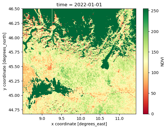
In the next episode, we will learn more about advanced visualization tools and how to make interactive plots using holoviews, a tool part of the HoloViz ecosystem.
Basic maths#
NDVI values are a little odd in comparison to standard NDVI range values [-1, +1]. This confirms the max values reported in the Product User Manual (PUM).
NDVI characteristics from the Product User Manual (PUM)#
layer name |
description |
physical min |
physical max |
digital max |
scaling |
offset |
No Data |
|---|---|---|---|---|---|---|---|
ndvi |
normalized difference vegetation index |
-0.08 |
0.92 |
250 |
1/250 |
-0.08 |
254, 255 |
ndvi_unc |
uncertainty on ndvi |
0 |
1 |
1000 |
1/1000 |
0 |
65535 |
nobs |
number of observations |
0 |
32 |
32 |
1 |
0 |
255 |
qflag |
bitwise quality flag |
- |
- |
254 |
1 |
0 |
255 |
from: Copernicus Global Land Service NDVI 300 V2.0.1
Simple arithmetic operations can be performed without worrying about dimensions and coordinates, using the same notation we use with numpy. Underneath xarray will automatically vectorize the operations over all the data dimensions.
NDVI_AOI * (1/250) - 0.08
<xarray.DataArray 'NDVI' (time: 20, lat: 612, lon: 984)>
array([[[0.94 , 0.94 , 0.94 , ..., 0.94 , 0.94 , 0.94 ],
        [0.94 , 0.94 , 0.94 , ..., 0.94 , 0.94 , 0.94 ],
        [0.94 , 0.94 , 0.94 , ..., 0.94 , 0.94 , 0.94 ],
        ...,
        [0.252, 0.32 , 0.316, ..., 0.416, 0.352, 0.94 ],
        [0.404, 0.4  , 0.368, ..., 0.416, 0.412, 0.94 ],
        [0.372, 0.292, 0.292, ..., 0.244, 0.4  , 0.94 ]],

       [[0.94 , 0.94 , 0.94 , ..., 0.94 , 0.508, 0.94 ],
        [0.94 , 0.94 , 0.94 , ..., 0.488, 0.48 , 0.94 ],
        [0.94 , 0.94 , 0.94 , ..., 0.444, 0.508, 0.94 ],
        ...,
        [0.472, 0.432, 0.416, ..., 0.484, 0.464, 0.94 ],
        [0.448, 0.412, 0.392, ..., 0.56 , 0.528, 0.94 ],
        [0.444, 0.424, 0.4  , ..., 0.484, 0.496, 0.94 ]],

       [[0.94 , 0.94 , 0.94 , ..., 0.496, 0.504, 0.94 ],
        [0.94 , 0.94 , 0.94 , ..., 0.5  , 0.496, 0.94 ],
        [0.94 , 0.94 , 0.94 , ..., 0.552, 0.52 , 0.94 ],
        ...,
...
        ...,
        [0.484, 0.484, 0.54 , ..., 0.424, 0.484, 0.94 ],
        [0.452, 0.424, 0.484, ..., 0.488, 0.52 , 0.94 ],
        [0.432, 0.408, 0.392, ..., 0.72 , 0.64 , 0.94 ]],

       [[0.768, 0.74 , 0.708, ..., 0.752, 0.768, 0.94 ],
        [0.7  , 0.724, 0.724, ..., 0.716, 0.748, 0.94 ],
        [0.776, 0.784, 0.788, ..., 0.728, 0.716, 0.94 ],
        ...,
        [0.54 , 0.56 , 0.604, ..., 0.268, 0.296, 0.94 ],
        [0.488, 0.52 , 0.536, ..., 0.448, 0.516, 0.94 ],
        [0.464, 0.48 , 0.532, ..., 0.564, 0.432, 0.94 ]],

       [[0.82 , 0.82 , 0.804, ..., 0.756, 0.756, 0.94 ],
        [0.712, 0.72 , 0.72 , ..., 0.764, 0.752, 0.94 ],
        [0.812, 0.848, 0.848, ..., 0.76 , 0.756, 0.94 ],
        ...,
        [0.58 , 0.568, 0.568, ..., 0.392, 0.4  , 0.94 ],
        [0.584, 0.532, 0.528, ..., 0.548, 0.548, 0.94 ],
        [0.556, 0.484, 0.488, ..., 0.62 , 0.584, 0.94 ]]])
Coordinates:
  * time     (time) datetime64[ns] 2022-01-01 2022-01-11 ... 2022-07-11
  * lon      (lon) float64 8.502 8.505 8.508 8.511 ... 11.42 11.42 11.42 11.43
* lat (lat) float64 46.5 46.5 46.49 46.49 ... 44.69 44.69 44.68 44.68The universal function (ufunc) from numpy and scipy can be applied too directly to the data.
np.subtract(np.multiply(NDVI_AOI, 0.004), 0.08)
<xarray.DataArray 'NDVI' (time: 20, lat: 612, lon: 984)>
array([[[0.94 , 0.94 , 0.94 , ..., 0.94 , 0.94 , 0.94 ],
        [0.94 , 0.94 , 0.94 , ..., 0.94 , 0.94 , 0.94 ],
        [0.94 , 0.94 , 0.94 , ..., 0.94 , 0.94 , 0.94 ],
        ...,
        [0.252, 0.32 , 0.316, ..., 0.416, 0.352, 0.94 ],
        [0.404, 0.4  , 0.368, ..., 0.416, 0.412, 0.94 ],
        [0.372, 0.292, 0.292, ..., 0.244, 0.4  , 0.94 ]],

       [[0.94 , 0.94 , 0.94 , ..., 0.94 , 0.508, 0.94 ],
        [0.94 , 0.94 , 0.94 , ..., 0.488, 0.48 , 0.94 ],
        [0.94 , 0.94 , 0.94 , ..., 0.444, 0.508, 0.94 ],
        ...,
        [0.472, 0.432, 0.416, ..., 0.484, 0.464, 0.94 ],
        [0.448, 0.412, 0.392, ..., 0.56 , 0.528, 0.94 ],
        [0.444, 0.424, 0.4  , ..., 0.484, 0.496, 0.94 ]],

       [[0.94 , 0.94 , 0.94 , ..., 0.496, 0.504, 0.94 ],
        [0.94 , 0.94 , 0.94 , ..., 0.5  , 0.496, 0.94 ],
        [0.94 , 0.94 , 0.94 , ..., 0.552, 0.52 , 0.94 ],
        ...,
...
        ...,
        [0.484, 0.484, 0.54 , ..., 0.424, 0.484, 0.94 ],
        [0.452, 0.424, 0.484, ..., 0.488, 0.52 , 0.94 ],
        [0.432, 0.408, 0.392, ..., 0.72 , 0.64 , 0.94 ]],

       [[0.768, 0.74 , 0.708, ..., 0.752, 0.768, 0.94 ],
        [0.7  , 0.724, 0.724, ..., 0.716, 0.748, 0.94 ],
        [0.776, 0.784, 0.788, ..., 0.728, 0.716, 0.94 ],
        ...,
        [0.54 , 0.56 , 0.604, ..., 0.268, 0.296, 0.94 ],
        [0.488, 0.52 , 0.536, ..., 0.448, 0.516, 0.94 ],
        [0.464, 0.48 , 0.532, ..., 0.564, 0.432, 0.94 ]],

       [[0.82 , 0.82 , 0.804, ..., 0.756, 0.756, 0.94 ],
        [0.712, 0.72 , 0.72 , ..., 0.764, 0.752, 0.94 ],
        [0.812, 0.848, 0.848, ..., 0.76 , 0.756, 0.94 ],
        ...,
        [0.58 , 0.568, 0.568, ..., 0.392, 0.4  , 0.94 ],
        [0.584, 0.532, 0.528, ..., 0.548, 0.548, 0.94 ],
        [0.556, 0.484, 0.488, ..., 0.62 , 0.584, 0.94 ]]])
Coordinates:
* time (time) datetime64[ns] 2022-01-01 2022-01-11 ... 2022-07-11
* lon (lon) float64 8.502 8.505 8.508 8.511 ... 11.42 11.42 11.42 11.43
* lat (lat) float64 46.5 46.5 46.49 46.49 ... 44.69 44.69 44.68 44.68
Attributes:
long_name: NDVI
units:
grid_mapping: crsNDVI_AOI = NDVI_AOI * (1/250) - 0.08
NDVI_AOI
<xarray.DataArray 'NDVI' (time: 20, lat: 612, lon: 984)>
array([[[0.94 , 0.94 , 0.94 , ..., 0.94 , 0.94 , 0.94 ],
        [0.94 , 0.94 , 0.94 , ..., 0.94 , 0.94 , 0.94 ],
        [0.94 , 0.94 , 0.94 , ..., 0.94 , 0.94 , 0.94 ],
        ...,
        [0.252, 0.32 , 0.316, ..., 0.416, 0.352, 0.94 ],
        [0.404, 0.4  , 0.368, ..., 0.416, 0.412, 0.94 ],
        [0.372, 0.292, 0.292, ..., 0.244, 0.4  , 0.94 ]],

       [[0.94 , 0.94 , 0.94 , ..., 0.94 , 0.508, 0.94 ],
        [0.94 , 0.94 , 0.94 , ..., 0.488, 0.48 , 0.94 ],
        [0.94 , 0.94 , 0.94 , ..., 0.444, 0.508, 0.94 ],
        ...,
        [0.472, 0.432, 0.416, ..., 0.484, 0.464, 0.94 ],
        [0.448, 0.412, 0.392, ..., 0.56 , 0.528, 0.94 ],
        [0.444, 0.424, 0.4  , ..., 0.484, 0.496, 0.94 ]],

       [[0.94 , 0.94 , 0.94 , ..., 0.496, 0.504, 0.94 ],
        [0.94 , 0.94 , 0.94 , ..., 0.5  , 0.496, 0.94 ],
        [0.94 , 0.94 , 0.94 , ..., 0.552, 0.52 , 0.94 ],
        ...,
...
        ...,
        [0.484, 0.484, 0.54 , ..., 0.424, 0.484, 0.94 ],
        [0.452, 0.424, 0.484, ..., 0.488, 0.52 , 0.94 ],
        [0.432, 0.408, 0.392, ..., 0.72 , 0.64 , 0.94 ]],

       [[0.768, 0.74 , 0.708, ..., 0.752, 0.768, 0.94 ],
        [0.7  , 0.724, 0.724, ..., 0.716, 0.748, 0.94 ],
        [0.776, 0.784, 0.788, ..., 0.728, 0.716, 0.94 ],
        ...,
        [0.54 , 0.56 , 0.604, ..., 0.268, 0.296, 0.94 ],
        [0.488, 0.52 , 0.536, ..., 0.448, 0.516, 0.94 ],
        [0.464, 0.48 , 0.532, ..., 0.564, 0.432, 0.94 ]],

       [[0.82 , 0.82 , 0.804, ..., 0.756, 0.756, 0.94 ],
        [0.712, 0.72 , 0.72 , ..., 0.764, 0.752, 0.94 ],
        [0.812, 0.848, 0.848, ..., 0.76 , 0.756, 0.94 ],
        ...,
        [0.58 , 0.568, 0.568, ..., 0.392, 0.4  , 0.94 ],
        [0.584, 0.532, 0.528, ..., 0.548, 0.548, 0.94 ],
        [0.556, 0.484, 0.488, ..., 0.62 , 0.584, 0.94 ]]])
Coordinates:
* time (time) datetime64[ns] 2022-01-01 2022-01-11 ... 2022-07-11
* lon (lon) float64 8.502 8.505 8.508 8.511 ... 11.42 11.42 11.42 11.43
* lat (lat) float64 46.5 46.5 46.49 46.49 ... 44.69 44.69 44.68 44.68Statistics#
All the standard statistical operations can be used such as min, max, mean. When no argument is passed to the function, the operation is done over all the dimension of the variable (same as with numpy).
NDVI_AOI.min()
<xarray.DataArray 'NDVI' ()>
array(-0.08)
You can make a statistical operation over a dimension. For instance, let’s retrieve the maximum value for each available time.
NDVI_AOI.max(dim='time')
<xarray.DataArray 'NDVI' (lat: 612, lon: 984)>
array([[0.94 , 0.94 , 0.94 , ..., 0.94 , 0.94 , 0.94 ],
       [0.94 , 0.94 , 0.94 , ..., 0.94 , 0.94 , 0.94 ],
       [0.94 , 0.94 , 0.94 , ..., 0.94 , 0.94 , 0.94 ],
       ...,
       [0.596, 0.584, 0.604, ..., 0.728, 0.804, 0.94 ],
       [0.584, 0.604, 0.588, ..., 0.708, 0.68 , 0.94 ],
       [0.556, 0.528, 0.532, ..., 0.72 , 0.64 , 0.94 ]])
Coordinates:
  * lon      (lon) float64 8.502 8.505 8.508 8.511 ... 11.42 11.42 11.42 11.43
* lat (lat) float64 46.5 46.5 46.49 46.49 ... 44.69 44.69 44.68 44.68Aggregation#
We have data every 10 days. To obtain monthly values, we can group values per month and compute the mean.
NDVI_monthly = NDVI_AOI.groupby(NDVI_AOI.time.dt.month).mean()
NDVI_monthly
<xarray.DataArray 'NDVI' (month: 7, lat: 612, lon: 984)>
array([[[0.94      , 0.94      , 0.94      , ..., 0.792     ,
         0.65066667, 0.94      ],
        [0.94      , 0.94      , 0.94      , ..., 0.64266667,
         0.63866667, 0.94      ],
        [0.94      , 0.94      , 0.94      , ..., 0.64533333,
         0.656     , 0.94      ],
        ...,
        [0.38666667, 0.39333333, 0.38666667, ..., 0.44133333,
         0.41866667, 0.94      ],
        [0.42533333, 0.40266667, 0.388     , ..., 0.47466667,
         0.464     , 0.94      ],
        [0.41066667, 0.388     , 0.372     , ..., 0.38666667,
         0.42533333, 0.94      ]],

       [[0.94      , 0.94      , 0.94      , ..., 0.46133333,
         0.468     , 0.94      ],
        [0.94      , 0.94      , 0.94      , ..., 0.44      ,
         0.41466667, 0.94      ],
        [0.94      , 0.94      , 0.94      , ..., 0.41466667,
         0.44933333, 0.94      ],
...
        [0.51866667, 0.52933333, 0.56133333, ..., 0.49066667,
         0.52666667, 0.94      ],
        [0.47733333, 0.49466667, 0.53733333, ..., 0.55333333,
         0.58533333, 0.94      ],
        [0.46266667, 0.41866667, 0.45733333, ..., 0.63333333,
         0.564     , 0.94      ]],

       [[0.794     , 0.78      , 0.756     , ..., 0.754     ,
         0.762     , 0.94      ],
        [0.706     , 0.722     , 0.722     , ..., 0.74      ,
         0.75      , 0.94      ],
        [0.794     , 0.816     , 0.818     , ..., 0.744     ,
         0.736     , 0.94      ],
        ...,
        [0.56      , 0.564     , 0.586     , ..., 0.33      ,
         0.348     , 0.94      ],
        [0.536     , 0.526     , 0.532     , ..., 0.498     ,
         0.532     , 0.94      ],
        [0.51      , 0.482     , 0.51      , ..., 0.592     ,
         0.508     , 0.94      ]]])
Coordinates:
  * lon      (lon) float64 8.502 8.505 8.508 8.511 ... 11.42 11.42 11.42 11.43
  * lat      (lat) float64 46.5 46.5 46.49 46.49 ... 44.69 44.69 44.68 44.68
* month (month) int64 1 2 3 4 5 6 7As we have data from January to July, the time dimension is now month and takes values from 1 to 7.
NDVI_monthly.month
<xarray.DataArray 'month' (month: 7)>
array([1, 2, 3, 4, 5, 6, 7])
Coordinates:
  * month    (month) int64 1 2 3 4 5 6 7
Mask#
Not all values are valid and masking all those which are not in the valid range [-0.08, 0.92] is necessary. Masking can be achieved through the method DataSet|Array.where(cond, other) or xr.where(cond, x, y).
The difference consists in the possibility to specify the value in case the condition is positive or not; DataSet|Array.where(cond, other) only offer the possibility to define the false condition value (by default is set to np.NaN))
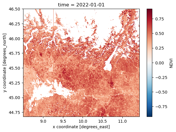
NDVI_masked = NDVI_AOI.where((NDVI_AOI >= -0.08) & (NDVI_AOI <= 0.92))
NDVI_masked.isel(time=0).plot()
<matplotlib.collections.QuadMesh at 0x7f0a2cc4bca0>
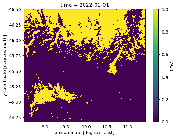
To better visualize the mask, with the help of xr.where, ad-hoc variable can be created. ‘xr.where’ let us specify value 1 for masked and 0 for the unmasked data.
mask = xr.where((NDVI_AOI <= -0.08) | (NDVI_AOI >= 0.92), 1, 0)
mask = xr.where((NDVI_AOI <= -0.08) | (NDVI_AOI >= 0.92), 1, 0)
mask.isel(time=0).plot()
<matplotlib.collections.QuadMesh at 0x7f0a2cb54340>
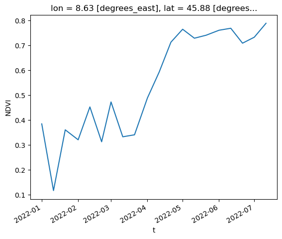
Plot a single point (defined by its latitude and longitude) over the time dimension.
NDVI_masked.sel(lat=45.88, lon=8.63, method='nearest').plot()
[<matplotlib.lines.Line2D at 0x7f0a2cbef3d0>]
Save xarray Dataset#
It is very often convenient to save intermediate or final results into a local file. We will learn more about the different file formats Xarray can handle, but for now let’s save it as a netCDF file. Check the file size after saving the result into netCDF.
NDVI_masked.to_netcdf('C_GLS_NDVI_20220101_20220701_Lombardia_S3_2_masked.nc')
Advance Saving methods#
Encoding and Compression#
From the NDVI dataset we already know that values can be encoded and can be conceptualized as pure Digital Numbers (DN). To revert those values to physical values (PhyVal) the formula PhyVal = DN * scale_factor + add_offset has to be used. To achieve the same result and transform our PhyVal back to DN 4 different parameters has to be defined :
dtype : datatype specification, in a numpy version (np.int16, np.float32) or a string one that can be converted to it. Here we use ‘np.uint8’ as values will range only up to 255.
_FillValues : a values that substitute the NaNs one. Some cast doesn’t allow the conversion of Nans as there is no physical representation for that value (like from Float to Int), so an alternative value withing the acceptable values needs to be specified.
scale_factor & add_offset : values can be converted through a scaling and off_set parameters according to the formula decoded = scale_factor * encoded + add_offset
A compression method can be defined as well; if the format is netCDF4 with the engine set to ‘netcdf4’ or ‘h5netcdf’ there are different compression options. The easiest solution is to stick with the default one for NetCDF4 files.
Note that encoding parameters needs to be done through a nested dictionary and parameters has to be defined for each single variable.
NDVI_masked.to_netcdf('C_GLS_NDVI_20220101_20220701_Lombardia_S3_2_mcs.nc',
                      engine='netcdf4',
                      encoding={'NDVI':{"dtype": np.uint8,
                                        '_FillValue': 255,
                                        'scale_factor':0.004,
                                        'add_offset':-0.08,
                                        'zlib': True, 'complevel':4}
                                }
                      )
- Xarray Dataset and DataArray
- Read and get metadata from local raster file
- Dataset and DataArray selection
- Aggregation and statistics
- Masking values
Through the datatype and the compression a compression of almost 10 time has been achieved; as drawback speed reading has been decreased.
References#
- Kog95
F.N. Kogan. Application of vegetation index and brightness temperature for drought detection. Advances in Space Research, 15(11):91–100, 1995. Natural Hazards: Monitoring and Assessment Using Remote Sensing Technique. URL: https://www.sciencedirect.com/science/article/pii/027311779500079T, doi:https://doi.org/10.1016/0273-1177(95)00079-T.
- Wik2)
Wikipedia. Normalized difference vegetation index. https://en.wikipedia.org/wiki/Normalized_difference_vegetation_index, 2022 (accessed August 7, 2022).
Packages citation#
- HMvdW+20
Charles R. Harris, K. Jarrod Millman, Stéfan J. van der Walt, Ralf Gommers, Pauli Virtanen, David Cournapeau, Eric Wieser, Julian Taylor, Sebastian Berg, Nathaniel J. Smith, Robert Kern, Matti Picus, Stephan Hoyer, Marten H. van Kerkwijk, Matthew Brett, Allan Haldane, Jaime Fernández del Río, Mark Wiebe, Pearu Peterson, Pierre Gérard-Marchant, Kevin Sheppard, Tyler Reddy, Warren Weckesser, Hameer Abbasi, Christoph Gohlke, and Travis E. Oliphant. Array programming with NumPy. Nature, 585(7825):357–362, September 2020. URL: https://doi.org/10.1038/s41586-020-2649-2, doi:10.1038/s41586-020-2649-2.
- HH17
S. Hoyer and J. Hamman. Xarray: N-D labeled arrays and datasets in Python. Journal of Open Research Software, 2017. URL: https://doi.org/10.5334/jors.148, doi:10.5334/jors.148.
- USR+20
Leonardo Uieda, Santiago Rubén Soler, Rémi Rampin, Hugo van Kemenade, Matthew Turk, Daniel Shapero, Anderson Banihirwe, and John Leeman. Pooch: a friend to fetch your data files. Journal of Open Source Software, 5(45):1943, 2020. URL: https://doi.org/10.21105/joss.01943, doi:10.21105/joss.01943.