Parallel computing with Dask on HPC (Spider Cluster SURF)

Authors & Contributors

Authors

• Tina Odaka, Ifremer (France), @tinaok

• Anne Fouilloux, Simula Research Laboratory (Norway), @annefou

• Francesco Nattino, Netherlands eScience Center (Netherlands), @fnattino

• Meiert W. Grootes, Netherlands eScience Center (Netherlands), @meiertgrootes

• Ou Ku, Netherlands eScience Center (Netherlands), @rogerkuou

Contributors

• Pier Lorenzo Marasco, Ispra (Italy), @pl-marasco

• Guillaume Eynard-Bontemps, CNES (France), @guillaumeeb

Overview

Questions

• What is Dask?
• How can I parallelize my data analysis with Dask?

Objectives

• Learn about Dask
• Learn about Dask Gateway, Dask Client, Scheduler, Workers
• Understand out-of-core and speed-up limitations

Context

We will be using Dask with Xarray to parallelize our data analysis. The analysis is very similar to what we have done in previous episodes but this time we will use data on a global coverage that we read from a shared catalog (stored online in the Pangeo EOSC Openstack Object Storage).

Data

In this episode, we will be using Global Long Term Statistics (1999-2019) product provided by the Copernicus Global Land Service over Lombardia and access them through S3-comptabile storage (OpenStack Object Storage “Swift”) with a data catalog we have created and made publicly available.

Setup

This episode uses the following Python packages:

• pooch [USR+20]

• s3fs [S3FsDTeam16]

• xarray [HH17] with netCDF4 and h5netcdf engines

• hvplot [RSB+20]

• dask [DaskDTeam16]

• graphviz [EGK+03]

• numpy [HMvdW+20]

• pandas [pdt20]

• geopandas [JdBF+20]

Please install these packages if not already available in your Python environment (you might want to take a look at the Setup info of the tutorial).

Packages

In this episode, Python packages are imported when we start to use them. However, for best software practices, we recommend you to install and import all the necessary libraries at the top of your Jupyter notebook.

Parallelize with Dask

We know from previous chapter chunking_introduction that chunking is key for analyzing large datasets. In this episode, we will learn to parallelize our data analysis using Dask on our chunked dataset.

What is Dask ?

Dask scales the existing Python ecosystem: with very or no changes in your code, you can speed-up computation using Dask or process bigger than memory datasets.

• Dask is a flexible library for parallel computing in Python.

• It is widely used for handling large and complex Earth Science datasets and speed up science.

• Dask is powerful, scalable and flexible. It is the leading platform today for data analytics at scale.

• It scales natively to clusters, cloud, HPC and bridges prototyping up to production.

• The strength of Dask is that is scales and accelerates the existing Python ecosystem e.g. Numpy, Pandas and Scikit-learn with few effort from end-users.

It is interesting to note that at first, Dask has been created to handle data that is larger than memory, on a single computer. It then was extended with Distributed to compute data in parallel over clusters of computers.

How does Dask scale and accelerate your data analysis?

Dask proposes different abstractions to distribute your computation. In this Dask Introduction section, we will focus on Dask Array which is widely used in pangeo ecosystem as a back end of Xarray.

As shown in the previous section Dask Array is based on chunks. Chunks of a Dask Array are well-known Numpy arrays. By transforming our big datasets to Dask Array, making use of chunk, a large array is handled as many smaller Numpy ones and we can compute each of these chunks independently.

Note

• `Xarray` uses Dask Arrays instead of Numpy when chunking is enabled, and thus all Xarray operations are performed through Dask, which enables distributed processing.

How does Xarray with Dask distribute data analysis?

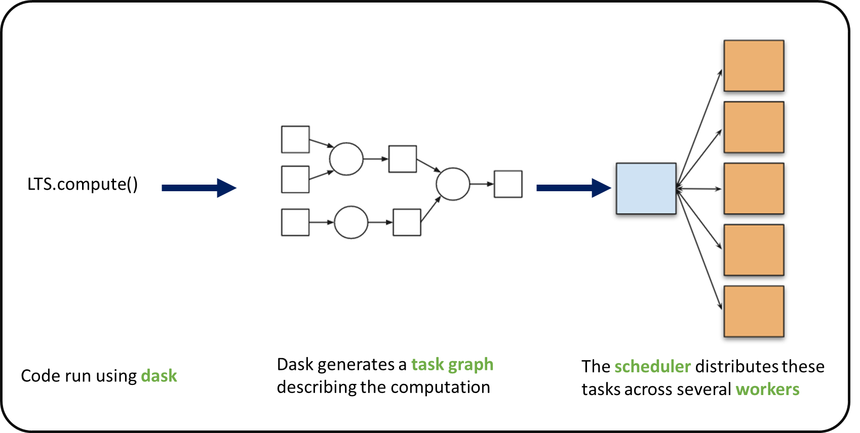
When we use chunks with Xarray, the real computation is only done when needed or asked for, usually when invoking compute() or load() functions. Dask generates a task graph describing the computations to be done. When using Dask Distributed a Scheduler distributes these tasks across several Workers.

What is a Dask Distributed cluster?

A Dask Distributed cluster is made of two main components:

• a Scheduler, responsible for handling computations graph and distributing tasks to Workers.

• One or several (up to 1000s) Workers, computing individual tasks and storing results and data into distributed memory (RAM and/or worker’s local disk).

A user usually needs Client and Cluster objects as shown below to use Dask Distributed.

Where can we deploy a Dask distributed cluster?

Dask distributed clusters can be deployed on your laptop or on distributed infrastructures (Cloud, HPC centers, Hadoop, etc.). Dask distributed Cluster object is responsible of deploying and scaling a Dask Cluster on the underlying resources.

Tip

A Dask Cluster can be created on a single machine (for instance your laptop) e.g. there is no need to have dedicated computational resources. However, speedup will only be limited to your single machine resources if you do not have dedicated computational resources!

Dask distributed Client

The Dask distributed Client is what allows you to interact with Dask distributed Clusters. When using Dask distributed, you always need to create a Client object. Once a Client has been created, it will be used by default by each call to a Dask API, even if you do not explicitly use it.

No matter the Dask API (e.g. Arrays, Dataframes, Delayed, Futures, etc.) that you use, under the hood, Dask will create a Directed Acyclic Graph (DAG) of tasks by analysing the code. Client will be responsible to submit this DAG to the Scheduler along with the final result you want to compute. The Client will also gather results from the Workers, and aggregate it back in its underlying Python process.

Using Client() function with no argument, you will create a local Dask cluster with a number of workers and threads per worker corresponding to the number of cores in the ‘local’ machine. Here, during the workshop, we are running this notebook in Pangeo EOSC cloud deployment, so the ‘local’ machine is the jupyterlab you are using at the Cloud, and the number of cores is the number of cores on the cloud computing resources you’ve been given (not on your laptop).

from dask.distributed import Client

client = Client()   # create a local dask cluster on the local machine.
client

/SPIDER_TYKKY_cmtWmSI/miniconda/envs/env1/lib/python3.11/site-packages/distributed/node.py:182: UserWarning: Port 8787 is already in use.
Perhaps you already have a cluster running?
Hosting the HTTP server on port 36415 instead
  warnings.warn(

Client

Client-2d1f81e3-349d-11ef-a4c8-fa163e5043d9

Connection method: Cluster object	Cluster type: distributed.LocalCluster
Dashboard: /proxy/36415/status

Launch dashboard in JupyterLab

Cluster Info

LocalCluster

1bfd1250

Dashboard: /proxy/36415/status	Workers: 4
Total threads: 4	Total memory: 31.25 GiB
Status: running	Using processes: True

Scheduler Info

Scheduler

Scheduler-a670b14f-eba5-41e5-921a-fa3a7bfb7b01

Comm: tcp://127.0.0.1:36983	Workers: 4
Dashboard: /proxy/36415/status	Total threads: 4
Started: Just now	Total memory: 31.25 GiB

Workers

Worker: 0

Comm: tcp://127.0.0.1:40121	Total threads: 1
Dashboard: /proxy/34251/status	Memory: 7.81 GiB
Nanny: tcp://127.0.0.1:41933
Local directory: /tmp/dask-scratch-space/worker-5q5s_887

Worker: 1

Comm: tcp://127.0.0.1:36907	Total threads: 1
Dashboard: /proxy/35967/status	Memory: 7.81 GiB
Nanny: tcp://127.0.0.1:38433
Local directory: /tmp/dask-scratch-space/worker-9flu0qmq

Worker: 2

Comm: tcp://127.0.0.1:41845	Total threads: 1
Dashboard: /proxy/42779/status	Memory: 7.81 GiB
Nanny: tcp://127.0.0.1:40805
Local directory: /tmp/dask-scratch-space/worker-dnpvrbba

Worker: 3

Comm: tcp://127.0.0.1:41873	Total threads: 1
Dashboard: /proxy/41387/status	Memory: 7.81 GiB
Nanny: tcp://127.0.0.1:37855
Local directory: /tmp/dask-scratch-space/worker-_h63ouyc

Inspecting the Cluster Info section above gives us information about the created cluster: we have 2 or 4 workers and the same number of threads (e.g. 1 thread per worker).

Go further

• You can also create a local cluster with the `LocalCluster` constructor and use `n_workers` and `threads_per_worker` to manually specify the number of processes and threads you want to use. For instance, we could use `n_workers=2` and `threads_per_worker=2`.
• This is sometimes preferable (in terms of performance), or when you run this tutorial on your PC, you can avoid dask to use all your resources you have on your PC!

Dask Dashboard

Dask comes with a really handy interface: the Dask Dashboard. It is a web interface that you can open in a separated tab of your browser (but not with he link above, you’ve got to use Jupyterlabs proxy: https://pangeo-eosc.vm.fedcloud.eu/jupyterhub/user/yourusername/proxy/8787/status).

We will learn here how to use it through dask jupyterlab extension.

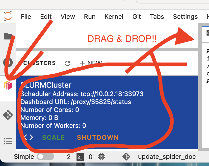
To use Dask Dashboard through jupyterlab extension on Pangeo EOSC infrastructure, you will just need too look at the html link you have for your jupyterlab, and Dask dashboard port number, as highlighted in the figure below.

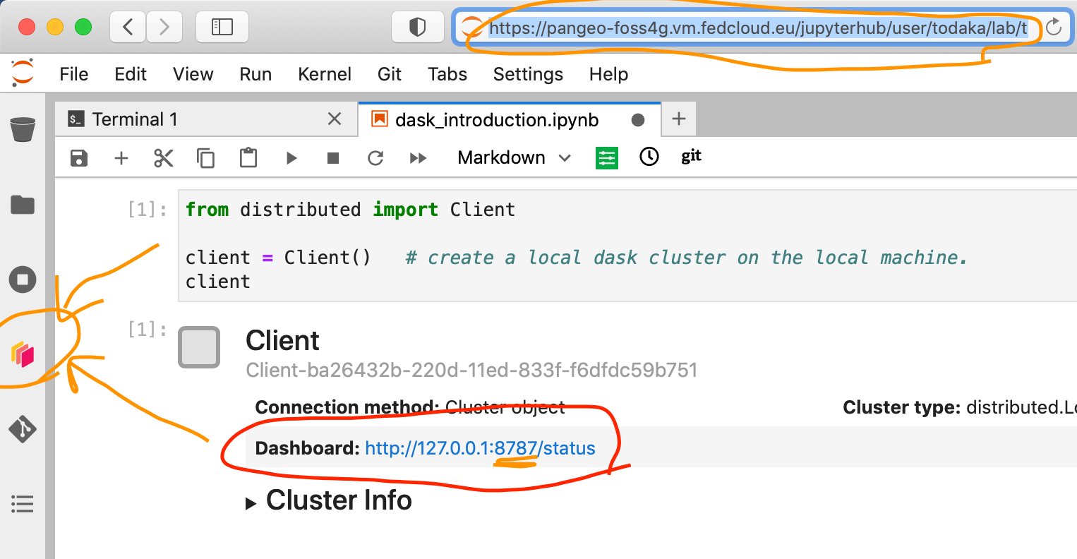
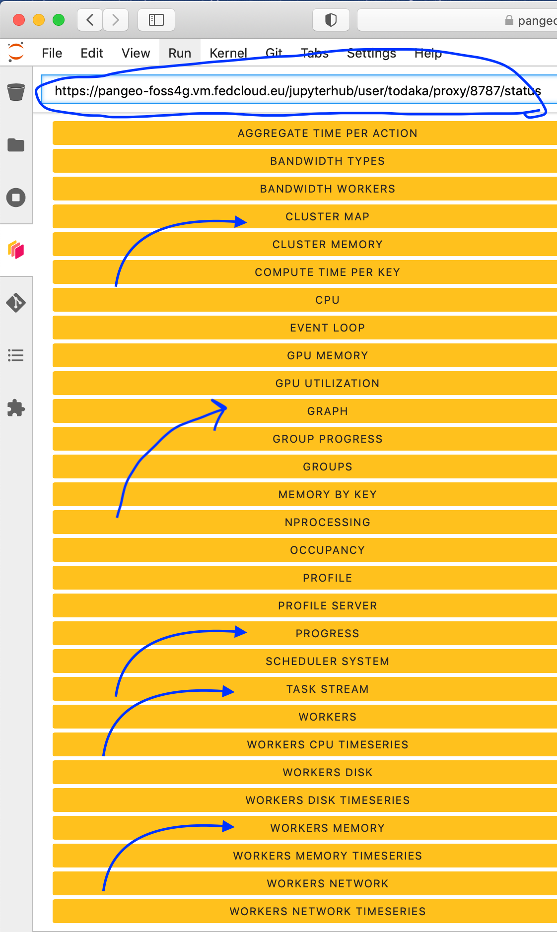
Then click the orange icon indicated in the above figure, and type ‘your’ dashboard link (normally, you just need to replace ‘todaka’ to ‘your username’).

You can click several buttons indicated with blue arrows in above figures, then drag and drop to place them as your convenience.

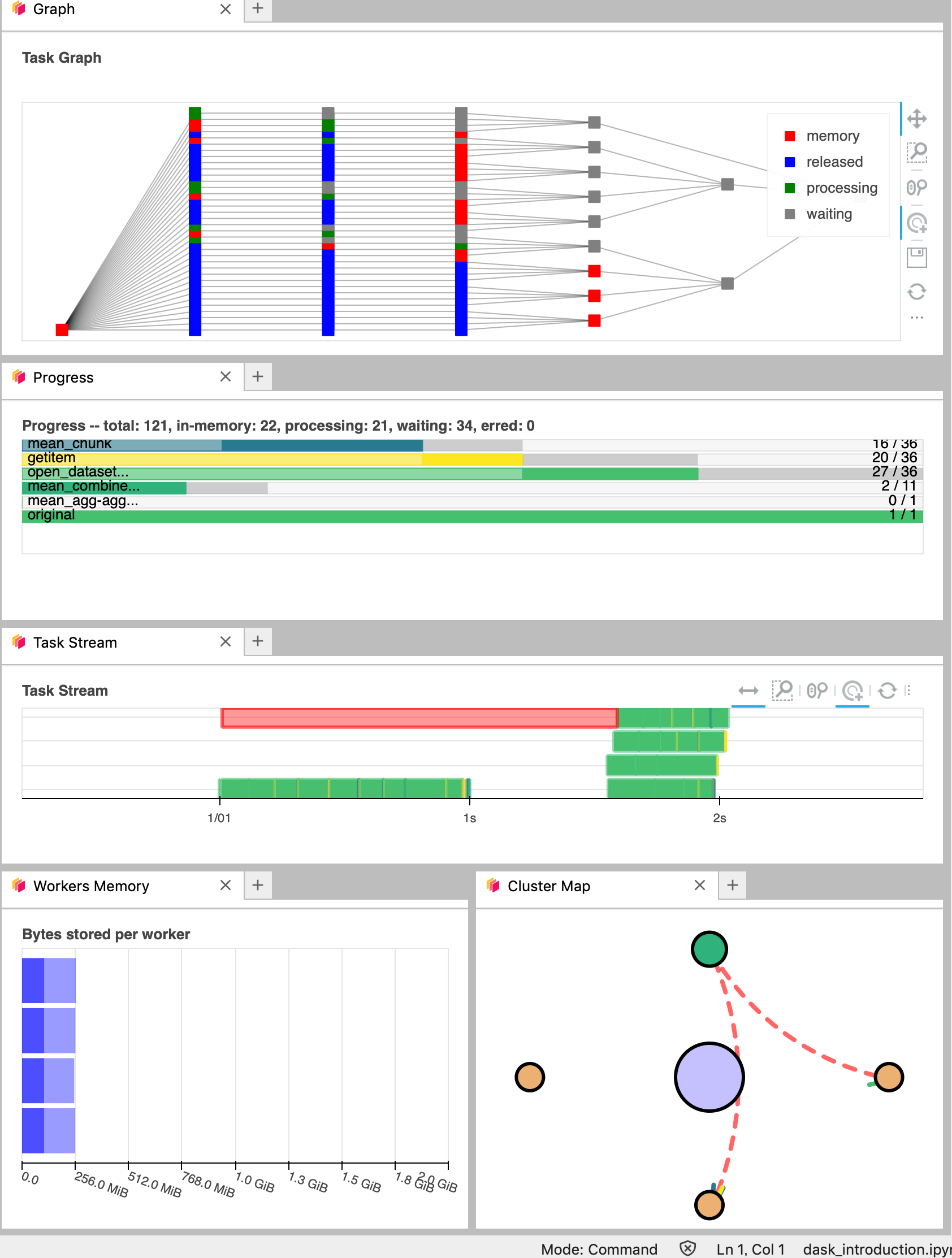
It’s really helpfull to understand your computation and how it is distributed.

Dask Distributed computations on our dataset

Let’s open the virtual dataset we’ve prepared as in previous episode, select a single location over time, visualize the task graph generated by Dask, and observe the Dask Dashboard.

Read from online kerchunked consolidated dataset

We will access Long Term TimeSeries of NDVI statistics from OpenStack Object Storage using the Zarr metadata generated with kerchunk, prepared in previous chunking_introduction section.

import xarray as xr

catalogue="https://pangeo-eosc-minioapi.vm.fedcloud.eu/afouilloux-ndvi/c_gls_NDVI-LTS_1999-2019.json"
LTS = xr.open_dataset(
    "reference://", engine="zarr",
    chunks={},
    backend_kwargs={
        "storage_options": {
            "fo": catalogue
                    },
        "consolidated": False
    }
)
LTS

/tmp/ipykernel_2991304/3611177325.py:4: UserWarning: Converting non-nanosecond precision datetime values to nanosecond precision. This behavior can eventually be relaxed in xarray, as it is an artifact from pandas which is now beginning to support non-nanosecond precision values. This warning is caused by passing non-nanosecond np.datetime64 or np.timedelta64 values to the DataArray or Variable constructor; it can be silenced by converting the values to nanosecond precision ahead of time.
  LTS = xr.open_dataset(
/tmp/ipykernel_2991304/3611177325.py:4: UserWarning: Converting non-nanosecond precision datetime values to nanosecond precision. This behavior can eventually be relaxed in xarray, as it is an artifact from pandas which is now beginning to support non-nanosecond precision values. This warning is caused by passing non-nanosecond np.datetime64 or np.timedelta64 values to the DataArray or Variable constructor; it can be silenced by converting the values to nanosecond precision ahead of time.
  LTS = xr.open_dataset(

<xarray.Dataset> Size: 1TB
Dimensions:  (lat: 15680, lon: 40320, time: 36)
Coordinates:
  * lat      (lat) float64 125kB 80.0 79.99 79.98 79.97 ... -59.97 -59.98 -59.99
  * lon      (lon) float64 323kB -180.0 -180.0 -180.0 ... 180.0 180.0 180.0
  * time     (time) datetime64[ns] 288B 2019-01-01 2019-01-11 ... 2019-12-21
Data variables:
    crs      object 8B ...
    max      (time, lat, lon) float64 182GB dask.array<chunksize=(1, 1207, 3102), meta=np.ndarray>
    mean     (time, lat, lon) float64 182GB dask.array<chunksize=(1, 1207, 3102), meta=np.ndarray>
    median   (time, lat, lon) float64 182GB dask.array<chunksize=(1, 1207, 3102), meta=np.ndarray>
    min      (time, lat, lon) float64 182GB dask.array<chunksize=(1, 1207, 3102), meta=np.ndarray>
    nobs     (time, lat, lon) float32 91GB dask.array<chunksize=(1, 1207, 3102), meta=np.ndarray>
    stdev    (time, lat, lon) float64 182GB dask.array<chunksize=(1, 1207, 3102), meta=np.ndarray>
Attributes: (12/19)
    Conventions:          CF-1.6
    archive_facility:     VITO
    copyright:            Copernicus Service information 2021
    history:              2021-03-01 - Processing line NDVI LTS
    identifier:           urn:cgls:global:ndvi_stats_all:NDVI-LTS_1999-2019-0...
    institution:          VITO NV
    ...                   ...
    references:           https://land.copernicus.eu/global/products/ndvi
    sensor:               VEGETATION-1, VEGETATION-2, VEGETATION
    source:               Derived from EO satellite imagery
    time_coverage_end:    2019-12-31T23:59:59Z
    time_coverage_start:  1999-01-01T00:00:00Z
    title:                Normalized Difference Vegetation Index: Long Term S...

xarray.Dataset

• Dimensions:
  • lat: 15680
  • lon: 40320
  • time: 36
• Coordinates: (3)
  • lat
    (lat)
    float64
    80.0 79.99 79.98 ... -59.98 -59.99

    DIMENSION_LABELS :

    lat

    _CoordinateAxisType :

    Lat

    axis :

    Y

    long_name :

    latitude

    standard_name :

    latitude

    units :

    degrees_north

    array([ 80.      ,  79.991071,  79.982143, ..., -59.973214, -59.982143,
           -59.991071])

  • lon
    (lon)
    float64
    -180.0 -180.0 ... 180.0 180.0

    DIMENSION_LABELS :

    lon

    _CoordinateAxisType :

    Lon

    axis :

    X

    long_name :

    longitude

    standard_name :

    longitude

    units :

    degrees_east

    array([-180.      , -179.991071, -179.982143, ...,  179.973214,  179.982143,
            179.991071])

  • time
    (time)
    datetime64[ns]
    2019-01-01 ... 2019-12-21

    _FillValue :

    1970-01-01T00:00:00

    array(['2019-01-01T00:00:00.000000000', '2019-01-11T00:00:00.000000000',
           '2019-01-21T00:00:00.000000000', '2019-02-01T00:00:00.000000000',
           '2019-02-11T00:00:00.000000000', '2019-02-21T00:00:00.000000000',
           '2019-03-01T00:00:00.000000000', '2019-03-11T00:00:00.000000000',
           '2019-03-21T00:00:00.000000000', '2019-04-01T00:00:00.000000000',
           '2019-04-11T00:00:00.000000000', '2019-04-21T00:00:00.000000000',
           '2019-05-01T00:00:00.000000000', '2019-05-11T00:00:00.000000000',
           '2019-05-21T00:00:00.000000000', '2019-06-01T00:00:00.000000000',
           '2019-06-11T00:00:00.000000000', '2019-06-21T00:00:00.000000000',
           '2019-07-01T00:00:00.000000000', '2019-07-11T00:00:00.000000000',
           '2019-07-21T00:00:00.000000000', '2019-08-01T00:00:00.000000000',
           '2019-08-11T00:00:00.000000000', '2019-08-21T00:00:00.000000000',
           '2019-09-01T00:00:00.000000000', '2019-09-11T00:00:00.000000000',
           '2019-09-21T00:00:00.000000000', '2019-10-01T00:00:00.000000000',
           '2019-10-11T00:00:00.000000000', '2019-10-21T00:00:00.000000000',
           '2019-11-01T00:00:00.000000000', '2019-11-11T00:00:00.000000000',
           '2019-11-21T00:00:00.000000000', '2019-12-01T00:00:00.000000000',
           '2019-12-11T00:00:00.000000000', '2019-12-21T00:00:00.000000000'],
          dtype='datetime64[ns]')

• Data variables: (7)
  • crs
    ()
    object
    ...

    GeoTransform :

    -180.0000000000 0.0089285714 0.0 80.0000000000 0.0 -0.0089285714

    _CoordinateAxisTypes :

    GeoX GeoY

    _CoordinateTransformType :

    Projection

    grid_mapping_name :

    latitude_longitude

    inverse_flattening :

    298.257223563

    long_name :

    coordinate reference system

    longitude_of_prime_meridian :

    0.0

    semi_major_axis :

    6378137.0

    spatial_ref :

    GEOGCS["WGS 84",DATUM["WGS_1984",SPHEROID["WGS 84",6378137,298.257223563,AUTHORITY["EPSG","7030"]],TOWGS84[0,0,0,0,0,0,0],AUTHORITY["EPSG","6326"]],PRIMEM["Greenwich",0,AUTHORITY["EPSG","8901"]],UNIT["degree",0.0174532925199433,AUTHORITY["EPSG","9108"]],AUTHORITY["EPSG","4326"]]

    [1 values with dtype=object]

  • max
    (time, lat, lon)
    float64
    dask.array<chunksize=(1, 1207, 3102), meta=np.ndarray>

    cell_methods :

    area: mean time: maximum

    flag_meanings :

    sea no_data

    flag_values :

    [254, 255]

    grid_mapping :

    crs

    long_name :

    Maximum Normalized Difference Vegetation Index over time period

    standard_name :

    normalized_difference_vegetation_index

    units :

    valid_range :

    [0, 250]

    Array Chunk Bytes 169.57 GiB 28.57 MiB Shape (36, 15680, 40320) (1, 1207, 3102) Dask graph 6084 chunks in 2 graph layers Data type float64 numpy.ndarray

  • mean
    (time, lat, lon)
    float64
    dask.array<chunksize=(1, 1207, 3102), meta=np.ndarray>

    cell_methods :

    area: mean time: mean

    flag_meanings :

    sea no_data

    flag_values :

    [254, 255]

    grid_mapping :

    crs

    long_name :

    Mean Normalized Difference Vegetation Index over time period

    standard_name :

    normalized_difference_vegetation_index

    units :

    valid_range :

    [0, 250]

    Array Chunk Bytes 169.57 GiB 28.57 MiB Shape (36, 15680, 40320) (1, 1207, 3102) Dask graph 6084 chunks in 2 graph layers Data type float64 numpy.ndarray

  • median
    (time, lat, lon)
    float64
    dask.array<chunksize=(1, 1207, 3102), meta=np.ndarray>

    cell_methods :

    area: mean time: median

    flag_meanings :

    sea no_data

    flag_values :

    [254, 255]

    grid_mapping :

    crs

    long_name :

    Median Normalized Difference Vegetation Index over time period

    standard_name :

    normalized_difference_vegetation_index

    units :

    valid_range :

    [0, 250]

    Array Chunk Bytes 169.57 GiB 28.57 MiB Shape (36, 15680, 40320) (1, 1207, 3102) Dask graph 6084 chunks in 2 graph layers Data type float64 numpy.ndarray

  • min
    (time, lat, lon)
    float64
    dask.array<chunksize=(1, 1207, 3102), meta=np.ndarray>

    cell_methods :

    area: mean time: minimum

    flag_meanings :

    sea no_data

    flag_values :

    [254, 255]

    grid_mapping :

    crs

    long_name :

    Minimum Normalized Difference Vegetation Index over time period

    standard_name :

    normalized_difference_vegetation_index

    units :

    valid_range :

    [0, 250]

    Array Chunk Bytes 169.57 GiB 28.57 MiB Shape (36, 15680, 40320) (1, 1207, 3102) Dask graph 6084 chunks in 2 graph layers Data type float64 numpy.ndarray

  • nobs
    (time, lat, lon)
    float32
    dask.array<chunksize=(1, 1207, 3102), meta=np.ndarray>

    cell_methods :

    area: mean

    grid_mapping :

    crs

    standard_name :

    normalized_difference_vegetation_index number_of_observations

    units :

    valid_range :

    [1, 250]

    Array Chunk Bytes 84.79 GiB 14.28 MiB Shape (36, 15680, 40320) (1, 1207, 3102) Dask graph 6084 chunks in 2 graph layers Data type float32 numpy.ndarray

  • stdev
    (time, lat, lon)
    float64
    dask.array<chunksize=(1, 1207, 3102), meta=np.ndarray>

    cell_methods :

    area: mean time: standard_deviation

    flag_meanings :

    sea no_data

    flag_values :

    [254, 255]

    grid_mapping :

    crs

    long_name :

    Standard deviation Normalized Difference Vegetation Index over time period

    standard_name :

    normalized_difference_vegetation_index

    units :

    valid_range :

    [0, 250]

    Array Chunk Bytes 169.57 GiB 28.57 MiB Shape (36, 15680, 40320) (1, 1207, 3102) Dask graph 6084 chunks in 2 graph layers Data type float64 numpy.ndarray

• Indexes: (3)
  • lat
    PandasIndex

    PandasIndex(Index([               80.0,   79.99107142857143,   79.98214285714286,
             79.97321428571429,   79.96428571428572,   79.95535714285715,
             79.94642857142858,   79.93750000000001,   79.92857142857144,
             79.91964285714288,
           ...
           -59.910714285682474,  -59.91964285711106,  -59.92857142853961,
            -59.93749999996817,  -59.94642857139675, -59.955357142825335,
            -59.96428571425389, -59.973214285682445,  -59.98214285711103,
            -59.99107142853961],
          dtype='float64', name='lat', length=15680))

  • lon
    PandasIndex

    PandasIndex(Index([             -180.0, -179.99107142857142, -179.98214285714283,
           -179.97321428571425, -179.96428571428567, -179.95535714285708,
            -179.9464285714285, -179.93749999999991, -179.92857142857133,
           -179.91964285714275,
           ...
             179.9107142862053,   179.9196428576339,  179.92857142906246,
              179.937500000491,  179.94642857191963,  179.95535714334824,
             179.9642857147768,  179.97321428620535,  179.98214285763396,
            179.99107142906257],
          dtype='float64', name='lon', length=40320))

  • time
    PandasIndex

    PandasIndex(DatetimeIndex(['2019-01-01', '2019-01-11', '2019-01-21', '2019-02-01',
                   '2019-02-11', '2019-02-21', '2019-03-01', '2019-03-11',
                   '2019-03-21', '2019-04-01', '2019-04-11', '2019-04-21',
                   '2019-05-01', '2019-05-11', '2019-05-21', '2019-06-01',
                   '2019-06-11', '2019-06-21', '2019-07-01', '2019-07-11',
                   '2019-07-21', '2019-08-01', '2019-08-11', '2019-08-21',
                   '2019-09-01', '2019-09-11', '2019-09-21', '2019-10-01',
                   '2019-10-11', '2019-10-21', '2019-11-01', '2019-11-11',
                   '2019-11-21', '2019-12-01', '2019-12-11', '2019-12-21'],
                  dtype='datetime64[s]', name='time', freq=None))

• Attributes: (19)

  Conventions :

  CF-1.6

  archive_facility :

  VITO

  copyright :

  Copernicus Service information 2021

  history :

  2021-03-01 - Processing line NDVI LTS

  identifier :

  urn:cgls:global:ndvi_stats_all:NDVI-LTS_1999-2019-0101_GLOBE_V3.0.1

  institution :

  VITO NV

  long_name :

  Normalized Difference Vegetation Index

  orbit_type :

  LEO

  parent_identifier :

  urn:cgls:global:ndvi_stats_all

  platform :

  SPOT-4, SPOT-5, Proba-V

  processing_level :

  L4

  processing_mode :

  Offline

  product_version :

  V3.0.1

  references :

  https://land.copernicus.eu/global/products/ndvi

  sensor :

  VEGETATION-1, VEGETATION-2, VEGETATION

  source :

  Derived from EO satellite imagery

  time_coverage_end :

  2019-12-31T23:59:59Z

  time_coverage_start :

  1999-01-01T00:00:00Z

  title :

  Normalized Difference Vegetation Index: Long Term Statistics 1KM: GLOBE 1999-2019 0101

By inspecting any of the variables on the representation above, you’ll see that each data array represents about 85GiB of data, so much more than the availabe memory on this notebook server, and even on the Dask Cluster we created above. But thanks to chunking, we can still analyze it!

save = LTS.sel(lat=45.50, lon=9.36, method='nearest')['min'].mean()
save.data

Array Chunk Bytes 8 B 8 B Shape () () Dask graph 1 chunks in 7 graph layers Data type float64 numpy.ndarray

Did you notice something on the Dask Dashboard when running the two previous cells?

We didn’t ‘compute’ anything. We just built a Dask task graph with it’s size indicated as count above, but did not ask Dask to return a result.

But the ‘task Count’ we see above is more than 6000 for just computing a mean on 36 temporal steps. This is too much. If you have such case, to avoid unecessary operations, you can optimize the task using dask.optimize.

Lets try to plot the dask graph before computation and understand what dask workers will do to compute the value we asked for.

Optimize the task graph

import dask
(save,) = dask.optimize(save)
save.data

Array Chunk Bytes 8 B 8 B Shape () () Dask graph 1 chunks in 1 graph layer Data type float64 numpy.ndarray

Now our task is reduced to about 100. Lets try to visualise it:

save.data.visualize()

Compute on the dask workers

save.compute()

<xarray.DataArray 'min' ()> Size: 8B
array(0.31844444)
Coordinates:
    lat      float64 8B 45.5
    lon      float64 8B 9.357

xarray.DataArray

'min'

• 0.3184

  array(0.31844444)

• Coordinates: (2)
  • lat
    ()
    float64
    45.5

    DIMENSION_LABELS :

    lat

    _CoordinateAxisType :

    Lat

    axis :

    Y

    long_name :

    latitude

    standard_name :

    latitude

    units :

    degrees_north

    array(45.5)

  • lon
    ()
    float64
    9.357

    DIMENSION_LABELS :

    lon

    _CoordinateAxisType :

    Lon

    axis :

    X

    long_name :

    longitude

    standard_name :

    longitude

    units :

    degrees_east

    array(9.35714286)

• Indexes: (0)
• Attributes: (0)

Calling compute on our Xarray object triggered the execution on Dask Cluster side.

You should be able to see how Dask is working on Dask Dashboard.

Go Further

• You can re-open the LTS with chunks=({"time":-1}) option, and try to visualize the task graph, size of each chunk, .... How did it changed? Do you see the difference of task graph using chunks keyword argument when opening the dataset?

Close client to terminate local dask cluster

The Client and associated LocalCluster object will be automatically closed when your Python session ends. When using Jupyter notebooks, we recommend to close it explicitely whenever you are done with your local Dask cluster.

client.close()

Scaling your Computation using Dask jobqueue.

For this workshop, according to the Pangeo EOSC deployment, you learned how to use Dask Gateway to manage Dask clusters over Kubernetes, allowing to run our data analysis in parallel e.g. distribute tasks across several workers.

Lets now try set up your Dask cluster using HPC infrastructure with Dask jobqueue.
As Dask jobqueue is configured by default on this ifnrastructure thanks to JupyterDaskOnSLURM we just installed in the last section, you just need drag & drop the SLURMCluster configuration cell, and execute it to connect the Dask jobqueue SLURMCluster.

from dask.distributed import Client

client = Client("tcp://10.0.0.65:37895")
client

Client

Client-aff498ad-349d-11ef-a4c8-fa163e5043d9

Connection method: Direct
Dashboard: /proxy/42841/status

Launch dashboard in JupyterLab

Scheduler Info

Scheduler

Scheduler-78b0cd43-aaca-4bec-a733-bfc4b1451f32

Comm: tcp://10.0.0.65:37895	Workers: 0
Dashboard: /proxy/42841/status	Total threads: 0
Started: 22 minutes ago	Total memory: 0 B

Workers

Make sure you use the right port (taken from the left panel), and click scale, to have several workers.

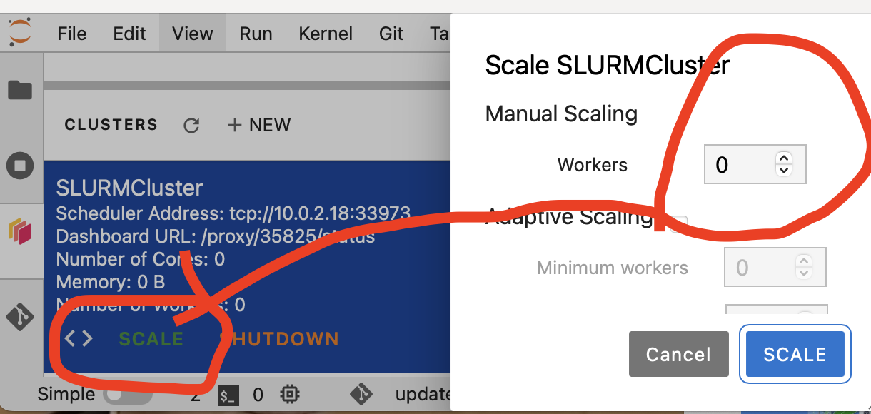
Adding a worker corresoinds to submiting a job using Slurm to start a node running a worker.

!squeue -u $USER

             JOBID PARTITION     NAME     USER ST       TIME  NODES NODELIST(REASON)
          13091627    normal dask-wor geocours  R       1:37      1 wn-ca-09
          13091628    normal dask-wor geocours  R       1:37      1 wn-dc-12
          13091629    normal dask-wor geocours  R       1:37      1 wn-ca-07
          13091630    normal dask-wor geocours  R       1:37      1 wn-ca-07
          13091613    normal jupyter_ geocours  R      26:08      1 wn-ca-03

Exercise

• The size of job you submitted is defined in your `~/.config/dask/config.yml`. Try updating it, to see how your resource (threads, memory size ...) changing after restarting your jupyter lab! (Observe well the dask dashboard!)

Global LTS computation

In the previous episode, we used Long-term Timeseries for the region of Lombardy e.g. a very small area that was extracted upfront for simplicity. Now we will use the original dataset that has a global coverage, and work directly on it to extract our AOI and perform computations.

Lets check our LTS data we have loaded before.

LTS

<xarray.Dataset> Size: 1TB
Dimensions:  (lat: 15680, lon: 40320, time: 36)
Coordinates:
  * lat      (lat) float64 125kB 80.0 79.99 79.98 79.97 ... -59.97 -59.98 -59.99
  * lon      (lon) float64 323kB -180.0 -180.0 -180.0 ... 180.0 180.0 180.0
  * time     (time) datetime64[ns] 288B 2022-01-01 2022-01-11 ... 2022-12-21
Data variables:
    crs      object 8B ...
    max      (time, lat, lon) float64 182GB dask.array<chunksize=(1, 1207, 3102), meta=np.ndarray>
    mean     (time, lat, lon) float64 182GB dask.array<chunksize=(1, 1207, 3102), meta=np.ndarray>
    median   (time, lat, lon) float64 182GB dask.array<chunksize=(1, 1207, 3102), meta=np.ndarray>
    min      (time, lat, lon) float64 182GB dask.array<chunksize=(1, 1207, 3102), meta=np.ndarray>
    nobs     (time, lat, lon) float32 91GB dask.array<chunksize=(1, 1207, 3102), meta=np.ndarray>
    stdev    (time, lat, lon) float64 182GB dask.array<chunksize=(1, 1207, 3102), meta=np.ndarray>
Attributes: (12/19)
    Conventions:          CF-1.6
    archive_facility:     VITO
    copyright:            Copernicus Service information 2021
    history:              2021-03-01 - Processing line NDVI LTS
    identifier:           urn:cgls:global:ndvi_stats_all:NDVI-LTS_1999-2019-0...
    institution:          VITO NV
    ...                   ...
    references:           https://land.copernicus.eu/global/products/ndvi
    sensor:               VEGETATION-1, VEGETATION-2, VEGETATION
    source:               Derived from EO satellite imagery
    time_coverage_end:    2019-12-31T23:59:59Z
    time_coverage_start:  1999-01-01T00:00:00Z
    title:                Normalized Difference Vegetation Index: Long Term S...

xarray.Dataset

• Dimensions:
  • lat: 15680
  • lon: 40320
  • time: 36
• Coordinates: (3)
  • lat
    (lat)
    float64
    80.0 79.99 79.98 ... -59.98 -59.99

    DIMENSION_LABELS :

    lat

    _CoordinateAxisType :

    Lat

    axis :

    Y

    long_name :

    latitude

    standard_name :

    latitude

    units :

    degrees_north

    array([ 80.      ,  79.991071,  79.982143, ..., -59.973214, -59.982143,
           -59.991071])

  • lon
    (lon)
    float64
    -180.0 -180.0 ... 180.0 180.0

    DIMENSION_LABELS :

    lon

    _CoordinateAxisType :

    Lon

    axis :

    X

    long_name :

    longitude

    standard_name :

    longitude

    units :

    degrees_east

    array([-180.      , -179.991071, -179.982143, ...,  179.973214,  179.982143,
            179.991071])

  • time
    (time)
    datetime64[ns]
    2022-01-01 ... 2022-12-21

    array(['2022-01-01T00:00:00.000000000', '2022-01-11T00:00:00.000000000',
           '2022-01-21T00:00:00.000000000', '2022-02-01T00:00:00.000000000',
           '2022-02-11T00:00:00.000000000', '2022-02-21T00:00:00.000000000',
           '2022-03-01T00:00:00.000000000', '2022-03-11T00:00:00.000000000',
           '2022-03-21T00:00:00.000000000', '2022-04-01T00:00:00.000000000',
           '2022-04-11T00:00:00.000000000', '2022-04-21T00:00:00.000000000',
           '2022-05-01T00:00:00.000000000', '2022-05-11T00:00:00.000000000',
           '2022-05-21T00:00:00.000000000', '2022-06-01T00:00:00.000000000',
           '2022-06-11T00:00:00.000000000', '2022-06-21T00:00:00.000000000',
           '2022-07-01T00:00:00.000000000', '2022-07-11T00:00:00.000000000',
           '2022-07-21T00:00:00.000000000', '2022-08-01T00:00:00.000000000',
           '2022-08-11T00:00:00.000000000', '2022-08-21T00:00:00.000000000',
           '2022-09-01T00:00:00.000000000', '2022-09-11T00:00:00.000000000',
           '2022-09-21T00:00:00.000000000', '2022-10-01T00:00:00.000000000',
           '2022-10-11T00:00:00.000000000', '2022-10-21T00:00:00.000000000',
           '2022-11-01T00:00:00.000000000', '2022-11-11T00:00:00.000000000',
           '2022-11-21T00:00:00.000000000', '2022-12-01T00:00:00.000000000',
           '2022-12-11T00:00:00.000000000', '2022-12-21T00:00:00.000000000'],
          dtype='datetime64[ns]')

• Data variables: (7)
  • crs
    ()
    object
    ...

    GeoTransform :

    -180.0000000000 0.0089285714 0.0 80.0000000000 0.0 -0.0089285714

    _CoordinateAxisTypes :

    GeoX GeoY

    _CoordinateTransformType :

    Projection

    grid_mapping_name :

    latitude_longitude

    inverse_flattening :

    298.257223563

    long_name :

    coordinate reference system

    longitude_of_prime_meridian :

    0.0

    semi_major_axis :

    6378137.0

    spatial_ref :

    GEOGCS["WGS 84",DATUM["WGS_1984",SPHEROID["WGS 84",6378137,298.257223563,AUTHORITY["EPSG","7030"]],TOWGS84[0,0,0,0,0,0,0],AUTHORITY["EPSG","6326"]],PRIMEM["Greenwich",0,AUTHORITY["EPSG","8901"]],UNIT["degree",0.0174532925199433,AUTHORITY["EPSG","9108"]],AUTHORITY["EPSG","4326"]]

    [1 values with dtype=object]

  • max
    (time, lat, lon)
    float64
    dask.array<chunksize=(1, 1207, 3102), meta=np.ndarray>

    cell_methods :

    area: mean time: maximum

    flag_meanings :

    sea no_data

    flag_values :

    [254, 255]

    grid_mapping :

    crs

    long_name :

    Maximum Normalized Difference Vegetation Index over time period

    standard_name :

    normalized_difference_vegetation_index

    units :

    valid_range :

    [0, 250]

    Array Chunk Bytes 169.57 GiB 28.57 MiB Shape (36, 15680, 40320) (1, 1207, 3102) Dask graph 6084 chunks in 2 graph layers Data type float64 numpy.ndarray

  • mean
    (time, lat, lon)
    float64
    dask.array<chunksize=(1, 1207, 3102), meta=np.ndarray>

    cell_methods :

    area: mean time: mean

    flag_meanings :

    sea no_data

    flag_values :

    [254, 255]

    grid_mapping :

    crs

    long_name :

    Mean Normalized Difference Vegetation Index over time period

    standard_name :

    normalized_difference_vegetation_index

    units :

    valid_range :

    [0, 250]

    Array Chunk Bytes 169.57 GiB 28.57 MiB Shape (36, 15680, 40320) (1, 1207, 3102) Dask graph 6084 chunks in 2 graph layers Data type float64 numpy.ndarray

  • median
    (time, lat, lon)
    float64
    dask.array<chunksize=(1, 1207, 3102), meta=np.ndarray>

    cell_methods :

    area: mean time: median

    flag_meanings :

    sea no_data

    flag_values :

    [254, 255]

    grid_mapping :

    crs

    long_name :

    Median Normalized Difference Vegetation Index over time period

    standard_name :

    normalized_difference_vegetation_index

    units :

    valid_range :

    [0, 250]

    Array Chunk Bytes 169.57 GiB 28.57 MiB Shape (36, 15680, 40320) (1, 1207, 3102) Dask graph 6084 chunks in 2 graph layers Data type float64 numpy.ndarray

  • min
    (time, lat, lon)
    float64
    dask.array<chunksize=(1, 1207, 3102), meta=np.ndarray>

    cell_methods :

    area: mean time: minimum

    flag_meanings :

    sea no_data

    flag_values :

    [254, 255]

    grid_mapping :

    crs

    long_name :

    Minimum Normalized Difference Vegetation Index over time period

    standard_name :

    normalized_difference_vegetation_index

    units :

    valid_range :

    [0, 250]

    Array Chunk Bytes 169.57 GiB 28.57 MiB Shape (36, 15680, 40320) (1, 1207, 3102) Dask graph 6084 chunks in 2 graph layers Data type float64 numpy.ndarray

  • nobs
    (time, lat, lon)
    float32
    dask.array<chunksize=(1, 1207, 3102), meta=np.ndarray>

    cell_methods :

    area: mean

    grid_mapping :

    crs

    standard_name :

    normalized_difference_vegetation_index number_of_observations

    units :

    valid_range :

    [1, 250]

    Array Chunk Bytes 84.79 GiB 14.28 MiB Shape (36, 15680, 40320) (1, 1207, 3102) Dask graph 6084 chunks in 2 graph layers Data type float32 numpy.ndarray

  • stdev
    (time, lat, lon)
    float64
    dask.array<chunksize=(1, 1207, 3102), meta=np.ndarray>

    cell_methods :

    area: mean time: standard_deviation

    flag_meanings :

    sea no_data

    flag_values :

    [254, 255]

    grid_mapping :

    crs

    long_name :

    Standard deviation Normalized Difference Vegetation Index over time period

    standard_name :

    normalized_difference_vegetation_index

    units :

    valid_range :

    [0, 250]

    Array Chunk Bytes 169.57 GiB 28.57 MiB Shape (36, 15680, 40320) (1, 1207, 3102) Dask graph 6084 chunks in 2 graph layers Data type float64 numpy.ndarray

• Indexes: (3)
  • lat
    PandasIndex

    PandasIndex(Index([               80.0,   79.99107142857143,   79.98214285714286,
             79.97321428571429,   79.96428571428572,   79.95535714285715,
             79.94642857142858,   79.93750000000001,   79.92857142857144,
             79.91964285714288,
           ...
           -59.910714285682474,  -59.91964285711106,  -59.92857142853961,
            -59.93749999996817,  -59.94642857139675, -59.955357142825335,
            -59.96428571425389, -59.973214285682445,  -59.98214285711103,
            -59.99107142853961],
          dtype='float64', name='lat', length=15680))

  • lon
    PandasIndex

    PandasIndex(Index([             -180.0, -179.99107142857142, -179.98214285714283,
           -179.97321428571425, -179.96428571428567, -179.95535714285708,
            -179.9464285714285, -179.93749999999991, -179.92857142857133,
           -179.91964285714275,
           ...
             179.9107142862053,   179.9196428576339,  179.92857142906246,
              179.937500000491,  179.94642857191963,  179.95535714334824,
             179.9642857147768,  179.97321428620535,  179.98214285763396,
            179.99107142906257],
          dtype='float64', name='lon', length=40320))

  • time
    PandasIndex

    PandasIndex(DatetimeIndex(['2022-01-01', '2022-01-11', '2022-01-21', '2022-02-01',
                   '2022-02-11', '2022-02-21', '2022-03-01', '2022-03-11',
                   '2022-03-21', '2022-04-01', '2022-04-11', '2022-04-21',
                   '2022-05-01', '2022-05-11', '2022-05-21', '2022-06-01',
                   '2022-06-11', '2022-06-21', '2022-07-01', '2022-07-11',
                   '2022-07-21', '2022-08-01', '2022-08-11', '2022-08-21',
                   '2022-09-01', '2022-09-11', '2022-09-21', '2022-10-01',
                   '2022-10-11', '2022-10-21', '2022-11-01', '2022-11-11',
                   '2022-11-21', '2022-12-01', '2022-12-11', '2022-12-21'],
                  dtype='datetime64[ns]', name='time', freq=None))

• Attributes: (19)

  Conventions :

  CF-1.6

  archive_facility :

  VITO

  copyright :

  Copernicus Service information 2021

  history :

  2021-03-01 - Processing line NDVI LTS

  identifier :

  urn:cgls:global:ndvi_stats_all:NDVI-LTS_1999-2019-0101_GLOBE_V3.0.1

  institution :

  VITO NV

  long_name :

  Normalized Difference Vegetation Index

  orbit_type :

  LEO

  parent_identifier :

  urn:cgls:global:ndvi_stats_all

  platform :

  SPOT-4, SPOT-5, Proba-V

  processing_level :

  L4

  processing_mode :

  Offline

  product_version :

  V3.0.1

  references :

  https://land.copernicus.eu/global/products/ndvi

  sensor :

  VEGETATION-1, VEGETATION-2, VEGETATION

  source :

  Derived from EO satellite imagery

  time_coverage_end :

  2019-12-31T23:59:59Z

  time_coverage_start :

  1999-01-01T00:00:00Z

  title :

  Normalized Difference Vegetation Index: Long Term Statistics 1KM: GLOBE 1999-2019 0101

Fix time coordinate

As observed data are coming with a predefined year. To let xarray automatically align the LTS with the lastest NDVI values, the time dimension needs to be shifted to the NDVI values.

import pandas as pd
import numpy as np

dates_2022 = pd.date_range('20220101', '20221231')
time_list = dates_2022[np.isin(dates_2022.day, [1,11,21])]
LTS = LTS.assign_coords(time=time_list)
LTS

<xarray.Dataset> Size: 1TB
Dimensions:  (lat: 15680, lon: 40320, time: 36)
Coordinates:
  * lat      (lat) float64 125kB 80.0 79.99 79.98 79.97 ... -59.97 -59.98 -59.99
  * lon      (lon) float64 323kB -180.0 -180.0 -180.0 ... 180.0 180.0 180.0
  * time     (time) datetime64[ns] 288B 2022-01-01 2022-01-11 ... 2022-12-21
Data variables:
    crs      object 8B ...
    max      (time, lat, lon) float64 182GB dask.array<chunksize=(1, 1207, 3102), meta=np.ndarray>
    mean     (time, lat, lon) float64 182GB dask.array<chunksize=(1, 1207, 3102), meta=np.ndarray>
    median   (time, lat, lon) float64 182GB dask.array<chunksize=(1, 1207, 3102), meta=np.ndarray>
    min      (time, lat, lon) float64 182GB dask.array<chunksize=(1, 1207, 3102), meta=np.ndarray>
    nobs     (time, lat, lon) float32 91GB dask.array<chunksize=(1, 1207, 3102), meta=np.ndarray>
    stdev    (time, lat, lon) float64 182GB dask.array<chunksize=(1, 1207, 3102), meta=np.ndarray>
Attributes: (12/19)
    Conventions:          CF-1.6
    archive_facility:     VITO
    copyright:            Copernicus Service information 2021
    history:              2021-03-01 - Processing line NDVI LTS
    identifier:           urn:cgls:global:ndvi_stats_all:NDVI-LTS_1999-2019-0...
    institution:          VITO NV
    ...                   ...
    references:           https://land.copernicus.eu/global/products/ndvi
    sensor:               VEGETATION-1, VEGETATION-2, VEGETATION
    source:               Derived from EO satellite imagery
    time_coverage_end:    2019-12-31T23:59:59Z
    time_coverage_start:  1999-01-01T00:00:00Z
    title:                Normalized Difference Vegetation Index: Long Term S...

xarray.Dataset

• Dimensions:
  • lat: 15680
  • lon: 40320
  • time: 36
• Coordinates: (3)
  • lat
    (lat)
    float64
    80.0 79.99 79.98 ... -59.98 -59.99

    DIMENSION_LABELS :

    lat

    _CoordinateAxisType :

    Lat

    axis :

    Y

    long_name :

    latitude

    standard_name :

    latitude

    units :

    degrees_north

    array([ 80.      ,  79.991071,  79.982143, ..., -59.973214, -59.982143,
           -59.991071])

  • lon
    (lon)
    float64
    -180.0 -180.0 ... 180.0 180.0

    DIMENSION_LABELS :

    lon

    _CoordinateAxisType :

    Lon

    axis :

    X

    long_name :

    longitude

    standard_name :

    longitude

    units :

    degrees_east

    array([-180.      , -179.991071, -179.982143, ...,  179.973214,  179.982143,
            179.991071])

  • time
    (time)
    datetime64[ns]
    2022-01-01 ... 2022-12-21

    array(['2022-01-01T00:00:00.000000000', '2022-01-11T00:00:00.000000000',
           '2022-01-21T00:00:00.000000000', '2022-02-01T00:00:00.000000000',
           '2022-02-11T00:00:00.000000000', '2022-02-21T00:00:00.000000000',
           '2022-03-01T00:00:00.000000000', '2022-03-11T00:00:00.000000000',
           '2022-03-21T00:00:00.000000000', '2022-04-01T00:00:00.000000000',
           '2022-04-11T00:00:00.000000000', '2022-04-21T00:00:00.000000000',
           '2022-05-01T00:00:00.000000000', '2022-05-11T00:00:00.000000000',
           '2022-05-21T00:00:00.000000000', '2022-06-01T00:00:00.000000000',
           '2022-06-11T00:00:00.000000000', '2022-06-21T00:00:00.000000000',
           '2022-07-01T00:00:00.000000000', '2022-07-11T00:00:00.000000000',
           '2022-07-21T00:00:00.000000000', '2022-08-01T00:00:00.000000000',
           '2022-08-11T00:00:00.000000000', '2022-08-21T00:00:00.000000000',
           '2022-09-01T00:00:00.000000000', '2022-09-11T00:00:00.000000000',
           '2022-09-21T00:00:00.000000000', '2022-10-01T00:00:00.000000000',
           '2022-10-11T00:00:00.000000000', '2022-10-21T00:00:00.000000000',
           '2022-11-01T00:00:00.000000000', '2022-11-11T00:00:00.000000000',
           '2022-11-21T00:00:00.000000000', '2022-12-01T00:00:00.000000000',
           '2022-12-11T00:00:00.000000000', '2022-12-21T00:00:00.000000000'],
          dtype='datetime64[ns]')

• Data variables: (7)
  • crs
    ()
    object
    ...

    GeoTransform :

    -180.0000000000 0.0089285714 0.0 80.0000000000 0.0 -0.0089285714

    _CoordinateAxisTypes :

    GeoX GeoY

    _CoordinateTransformType :

    Projection

    grid_mapping_name :

    latitude_longitude

    inverse_flattening :

    298.257223563

    long_name :

    coordinate reference system

    longitude_of_prime_meridian :

    0.0

    semi_major_axis :

    6378137.0

    spatial_ref :

    GEOGCS["WGS 84",DATUM["WGS_1984",SPHEROID["WGS 84",6378137,298.257223563,AUTHORITY["EPSG","7030"]],TOWGS84[0,0,0,0,0,0,0],AUTHORITY["EPSG","6326"]],PRIMEM["Greenwich",0,AUTHORITY["EPSG","8901"]],UNIT["degree",0.0174532925199433,AUTHORITY["EPSG","9108"]],AUTHORITY["EPSG","4326"]]

    [1 values with dtype=object]

  • max
    (time, lat, lon)
    float64
    dask.array<chunksize=(1, 1207, 3102), meta=np.ndarray>

    cell_methods :

    area: mean time: maximum

    flag_meanings :

    sea no_data

    flag_values :

    [254, 255]

    grid_mapping :

    crs

    long_name :

    Maximum Normalized Difference Vegetation Index over time period

    standard_name :

    normalized_difference_vegetation_index

    units :

    valid_range :

    [0, 250]

    Array Chunk Bytes 169.57 GiB 28.57 MiB Shape (36, 15680, 40320) (1, 1207, 3102) Dask graph 6084 chunks in 2 graph layers Data type float64 numpy.ndarray

  • mean
    (time, lat, lon)
    float64
    dask.array<chunksize=(1, 1207, 3102), meta=np.ndarray>

    cell_methods :

    area: mean time: mean

    flag_meanings :

    sea no_data

    flag_values :

    [254, 255]

    grid_mapping :

    crs

    long_name :

    Mean Normalized Difference Vegetation Index over time period

    standard_name :

    normalized_difference_vegetation_index

    units :

    valid_range :

    [0, 250]

    Array Chunk Bytes 169.57 GiB 28.57 MiB Shape (36, 15680, 40320) (1, 1207, 3102) Dask graph 6084 chunks in 2 graph layers Data type float64 numpy.ndarray

  • median
    (time, lat, lon)
    float64
    dask.array<chunksize=(1, 1207, 3102), meta=np.ndarray>

    cell_methods :

    area: mean time: median

    flag_meanings :

    sea no_data

    flag_values :

    [254, 255]

    grid_mapping :

    crs

    long_name :

    Median Normalized Difference Vegetation Index over time period

    standard_name :

    normalized_difference_vegetation_index

    units :

    valid_range :

    [0, 250]

    Array Chunk Bytes 169.57 GiB 28.57 MiB Shape (36, 15680, 40320) (1, 1207, 3102) Dask graph 6084 chunks in 2 graph layers Data type float64 numpy.ndarray

  • min
    (time, lat, lon)
    float64
    dask.array<chunksize=(1, 1207, 3102), meta=np.ndarray>

    cell_methods :

    area: mean time: minimum

    flag_meanings :

    sea no_data

    flag_values :

    [254, 255]

    grid_mapping :

    crs

    long_name :

    Minimum Normalized Difference Vegetation Index over time period

    standard_name :

    normalized_difference_vegetation_index

    units :

    valid_range :

    [0, 250]

    Array Chunk Bytes 169.57 GiB 28.57 MiB Shape (36, 15680, 40320) (1, 1207, 3102) Dask graph 6084 chunks in 2 graph layers Data type float64 numpy.ndarray

  • nobs
    (time, lat, lon)
    float32
    dask.array<chunksize=(1, 1207, 3102), meta=np.ndarray>

    cell_methods :

    area: mean

    grid_mapping :

    crs

    standard_name :

    normalized_difference_vegetation_index number_of_observations

    units :

    valid_range :

    [1, 250]

    Array Chunk Bytes 84.79 GiB 14.28 MiB Shape (36, 15680, 40320) (1, 1207, 3102) Dask graph 6084 chunks in 2 graph layers Data type float32 numpy.ndarray

  • stdev
    (time, lat, lon)
    float64
    dask.array<chunksize=(1, 1207, 3102), meta=np.ndarray>

    cell_methods :

    area: mean time: standard_deviation

    flag_meanings :

    sea no_data

    flag_values :

    [254, 255]

    grid_mapping :

    crs

    long_name :

    Standard deviation Normalized Difference Vegetation Index over time period

    standard_name :

    normalized_difference_vegetation_index

    units :

    valid_range :

    [0, 250]

    Array Chunk Bytes 169.57 GiB 28.57 MiB Shape (36, 15680, 40320) (1, 1207, 3102) Dask graph 6084 chunks in 2 graph layers Data type float64 numpy.ndarray

• Indexes: (3)
  • lat
    PandasIndex

    PandasIndex(Index([               80.0,   79.99107142857143,   79.98214285714286,
             79.97321428571429,   79.96428571428572,   79.95535714285715,
             79.94642857142858,   79.93750000000001,   79.92857142857144,
             79.91964285714288,
           ...
           -59.910714285682474,  -59.91964285711106,  -59.92857142853961,
            -59.93749999996817,  -59.94642857139675, -59.955357142825335,
            -59.96428571425389, -59.973214285682445,  -59.98214285711103,
            -59.99107142853961],
          dtype='float64', name='lat', length=15680))

  • lon
    PandasIndex

    PandasIndex(Index([             -180.0, -179.99107142857142, -179.98214285714283,
           -179.97321428571425, -179.96428571428567, -179.95535714285708,
            -179.9464285714285, -179.93749999999991, -179.92857142857133,
           -179.91964285714275,
           ...
             179.9107142862053,   179.9196428576339,  179.92857142906246,
              179.937500000491,  179.94642857191963,  179.95535714334824,
             179.9642857147768,  179.97321428620535,  179.98214285763396,
            179.99107142906257],
          dtype='float64', name='lon', length=40320))

  • time
    PandasIndex

    PandasIndex(DatetimeIndex(['2022-01-01', '2022-01-11', '2022-01-21', '2022-02-01',
                   '2022-02-11', '2022-02-21', '2022-03-01', '2022-03-11',
                   '2022-03-21', '2022-04-01', '2022-04-11', '2022-04-21',
                   '2022-05-01', '2022-05-11', '2022-05-21', '2022-06-01',
                   '2022-06-11', '2022-06-21', '2022-07-01', '2022-07-11',
                   '2022-07-21', '2022-08-01', '2022-08-11', '2022-08-21',
                   '2022-09-01', '2022-09-11', '2022-09-21', '2022-10-01',
                   '2022-10-11', '2022-10-21', '2022-11-01', '2022-11-11',
                   '2022-11-21', '2022-12-01', '2022-12-11', '2022-12-21'],
                  dtype='datetime64[ns]', name='time', freq=None))

• Attributes: (19)

  Conventions :

  CF-1.6

  archive_facility :

  VITO

  copyright :

  Copernicus Service information 2021

  history :

  2021-03-01 - Processing line NDVI LTS

  identifier :

  urn:cgls:global:ndvi_stats_all:NDVI-LTS_1999-2019-0101_GLOBE_V3.0.1

  institution :

  VITO NV

  long_name :

  Normalized Difference Vegetation Index

  orbit_type :

  LEO

  parent_identifier :

  urn:cgls:global:ndvi_stats_all

  platform :

  SPOT-4, SPOT-5, Proba-V

  processing_level :

  L4

  processing_mode :

  Offline

  product_version :

  V3.0.1

  references :

  https://land.copernicus.eu/global/products/ndvi

  sensor :

  VEGETATION-1, VEGETATION-2, VEGETATION

  source :

  Derived from EO satellite imagery

  time_coverage_end :

  2019-12-31T23:59:59Z

  time_coverage_start :

  1999-01-01T00:00:00Z

  title :

  Normalized Difference Vegetation Index: Long Term Statistics 1KM: GLOBE 1999-2019 0101

Clip LTS over Lombardia

As in previous episodes, we use a shapefile over Italy to select data over this Area of Interest (AOI).

import geopandas as gpd
GAUL = gpd.read_file('Italy.geojson')

AOI_name = 'Lombardia'
AOI = GAUL[GAUL.name1 == AOI_name]
AOI_poly = AOI.geometry
AOI_poly

14    POLYGON ((10.23973 46.62177, 10.25084 46.6111,...
Name: geometry, dtype: geometry

We first select a geographical area that covers Lombardia (so that we have a first reduction from the global coverage) and then clip using the shapefile to avoid useless pixels.

LTS_AOI = LTS.sel(lat=slice(46.5,44.5), lon=slice(8.5,11.5))
LTS_AOI.rio.write_crs(4326, inplace=True)

<xarray.Dataset> Size: 119MB
Dimensions:  (lat: 224, lon: 336, time: 36)
Coordinates:
    crs      int64 8B 0
  * lat      (lat) float64 2kB 46.49 46.48 46.47 46.46 ... 44.52 44.51 44.5
  * lon      (lon) float64 3kB 8.5 8.509 8.518 8.527 ... 11.46 11.47 11.48 11.49
  * time     (time) datetime64[ns] 288B 2022-01-01 2022-01-11 ... 2022-12-21
Data variables:
    max      (time, lat, lon) float64 22MB dask.array<chunksize=(1, 224, 336), meta=np.ndarray>
    mean     (time, lat, lon) float64 22MB dask.array<chunksize=(1, 224, 336), meta=np.ndarray>
    median   (time, lat, lon) float64 22MB dask.array<chunksize=(1, 224, 336), meta=np.ndarray>
    min      (time, lat, lon) float64 22MB dask.array<chunksize=(1, 224, 336), meta=np.ndarray>
    nobs     (time, lat, lon) float32 11MB dask.array<chunksize=(1, 224, 336), meta=np.ndarray>
    stdev    (time, lat, lon) float64 22MB dask.array<chunksize=(1, 224, 336), meta=np.ndarray>
Attributes: (12/19)
    Conventions:          CF-1.6
    archive_facility:     VITO
    copyright:            Copernicus Service information 2021
    history:              2021-03-01 - Processing line NDVI LTS
    identifier:           urn:cgls:global:ndvi_stats_all:NDVI-LTS_1999-2019-0...
    institution:          VITO NV
    ...                   ...
    references:           https://land.copernicus.eu/global/products/ndvi
    sensor:               VEGETATION-1, VEGETATION-2, VEGETATION
    source:               Derived from EO satellite imagery
    time_coverage_end:    2019-12-31T23:59:59Z
    time_coverage_start:  1999-01-01T00:00:00Z
    title:                Normalized Difference Vegetation Index: Long Term S...

xarray.Dataset

• Dimensions:
  • lat: 224
  • lon: 336
  • time: 36
• Coordinates: (4)
  • crs
    ()
    int64
    0

    crs_wkt :

    GEOGCS["WGS 84",DATUM["WGS_1984",SPHEROID["WGS 84",6378137,298.257223563,AUTHORITY["EPSG","7030"]],AUTHORITY["EPSG","6326"]],PRIMEM["Greenwich",0,AUTHORITY["EPSG","8901"]],UNIT["degree",0.0174532925199433,AUTHORITY["EPSG","9122"]],AXIS["Latitude",NORTH],AXIS["Longitude",EAST],AUTHORITY["EPSG","4326"]]

    semi_major_axis :

    6378137.0

    semi_minor_axis :

    6356752.314245179

    inverse_flattening :

    298.257223563

    reference_ellipsoid_name :

    WGS 84

    longitude_of_prime_meridian :

    0.0

    prime_meridian_name :

    Greenwich

    geographic_crs_name :

    WGS 84

    horizontal_datum_name :

    World Geodetic System 1984

    grid_mapping_name :

    latitude_longitude

    spatial_ref :

    GEOGCS["WGS 84",DATUM["WGS_1984",SPHEROID["WGS 84",6378137,298.257223563,AUTHORITY["EPSG","7030"]],AUTHORITY["EPSG","6326"]],PRIMEM["Greenwich",0,AUTHORITY["EPSG","8901"]],UNIT["degree",0.0174532925199433,AUTHORITY["EPSG","9122"]],AXIS["Latitude",NORTH],AXIS["Longitude",EAST],AUTHORITY["EPSG","4326"]]

    array(0)

  • lat
    (lat)
    float64
    46.49 46.48 46.47 ... 44.51 44.5

    DIMENSION_LABELS :

    lat

    _CoordinateAxisType :

    Lat

    axis :

    Y

    long_name :

    latitude

    standard_name :

    latitude

    units :

    degrees_north

    array([46.491071, 46.482143, 46.473214, ..., 44.517857, 44.508929, 44.5     ])

  • lon
    (lon)
    float64
    8.5 8.509 8.518 ... 11.48 11.49

    DIMENSION_LABELS :

    lon

    _CoordinateAxisType :

    Lon

    axis :

    X

    long_name :

    longitude

    standard_name :

    longitude

    units :

    degrees_east

    array([ 8.5     ,  8.508929,  8.517857, ..., 11.473214, 11.482143, 11.491071])

  • time
    (time)
    datetime64[ns]
    2022-01-01 ... 2022-12-21

    array(['2022-01-01T00:00:00.000000000', '2022-01-11T00:00:00.000000000',
           '2022-01-21T00:00:00.000000000', '2022-02-01T00:00:00.000000000',
           '2022-02-11T00:00:00.000000000', '2022-02-21T00:00:00.000000000',
           '2022-03-01T00:00:00.000000000', '2022-03-11T00:00:00.000000000',
           '2022-03-21T00:00:00.000000000', '2022-04-01T00:00:00.000000000',
           '2022-04-11T00:00:00.000000000', '2022-04-21T00:00:00.000000000',
           '2022-05-01T00:00:00.000000000', '2022-05-11T00:00:00.000000000',
           '2022-05-21T00:00:00.000000000', '2022-06-01T00:00:00.000000000',
           '2022-06-11T00:00:00.000000000', '2022-06-21T00:00:00.000000000',
           '2022-07-01T00:00:00.000000000', '2022-07-11T00:00:00.000000000',
           '2022-07-21T00:00:00.000000000', '2022-08-01T00:00:00.000000000',
           '2022-08-11T00:00:00.000000000', '2022-08-21T00:00:00.000000000',
           '2022-09-01T00:00:00.000000000', '2022-09-11T00:00:00.000000000',
           '2022-09-21T00:00:00.000000000', '2022-10-01T00:00:00.000000000',
           '2022-10-11T00:00:00.000000000', '2022-10-21T00:00:00.000000000',
           '2022-11-01T00:00:00.000000000', '2022-11-11T00:00:00.000000000',
           '2022-11-21T00:00:00.000000000', '2022-12-01T00:00:00.000000000',
           '2022-12-11T00:00:00.000000000', '2022-12-21T00:00:00.000000000'],
          dtype='datetime64[ns]')

• Data variables: (6)
  • max
    (time, lat, lon)
    float64
    dask.array<chunksize=(1, 224, 336), meta=np.ndarray>

    cell_methods :

    area: mean time: maximum

    flag_meanings :

    sea no_data

    flag_values :

    [254, 255]

    long_name :

    Maximum Normalized Difference Vegetation Index over time period

    standard_name :

    normalized_difference_vegetation_index

    units :

    valid_range :

    [0, 250]

    Array Chunk Bytes 20.67 MiB 588.00 kiB Shape (36, 224, 336) (1, 224, 336) Dask graph 36 chunks in 3 graph layers Data type float64 numpy.ndarray

  • mean
    (time, lat, lon)
    float64
    dask.array<chunksize=(1, 224, 336), meta=np.ndarray>

    cell_methods :

    area: mean time: mean

    flag_meanings :

    sea no_data

    flag_values :

    [254, 255]

    long_name :

    Mean Normalized Difference Vegetation Index over time period

    standard_name :

    normalized_difference_vegetation_index

    units :

    valid_range :

    [0, 250]

    Array Chunk Bytes 20.67 MiB 588.00 kiB Shape (36, 224, 336) (1, 224, 336) Dask graph 36 chunks in 3 graph layers Data type float64 numpy.ndarray

  • median
    (time, lat, lon)
    float64
    dask.array<chunksize=(1, 224, 336), meta=np.ndarray>

    cell_methods :

    area: mean time: median

    flag_meanings :

    sea no_data

    flag_values :

    [254, 255]

    long_name :

    Median Normalized Difference Vegetation Index over time period

    standard_name :

    normalized_difference_vegetation_index

    units :

    valid_range :

    [0, 250]

    Array Chunk Bytes 20.67 MiB 588.00 kiB Shape (36, 224, 336) (1, 224, 336) Dask graph 36 chunks in 3 graph layers Data type float64 numpy.ndarray

  • min
    (time, lat, lon)
    float64
    dask.array<chunksize=(1, 224, 336), meta=np.ndarray>

    cell_methods :

    area: mean time: minimum

    flag_meanings :

    sea no_data

    flag_values :

    [254, 255]

    long_name :

    Minimum Normalized Difference Vegetation Index over time period

    standard_name :

    normalized_difference_vegetation_index

    units :

    valid_range :

    [0, 250]

    Array Chunk Bytes 20.67 MiB 588.00 kiB Shape (36, 224, 336) (1, 224, 336) Dask graph 36 chunks in 3 graph layers Data type float64 numpy.ndarray

  • nobs
    (time, lat, lon)
    float32
    dask.array<chunksize=(1, 224, 336), meta=np.ndarray>

    cell_methods :

    area: mean

    standard_name :

    normalized_difference_vegetation_index number_of_observations

    units :

    valid_range :

    [1, 250]

    Array Chunk Bytes 10.34 MiB 294.00 kiB Shape (36, 224, 336) (1, 224, 336) Dask graph 36 chunks in 3 graph layers Data type float32 numpy.ndarray

  • stdev
    (time, lat, lon)
    float64
    dask.array<chunksize=(1, 224, 336), meta=np.ndarray>

    cell_methods :

    area: mean time: standard_deviation

    flag_meanings :

    sea no_data

    flag_values :

    [254, 255]

    long_name :

    Standard deviation Normalized Difference Vegetation Index over time period

    standard_name :

    normalized_difference_vegetation_index

    units :

    valid_range :

    [0, 250]

    Array Chunk Bytes 20.67 MiB 588.00 kiB Shape (36, 224, 336) (1, 224, 336) Dask graph 36 chunks in 3 graph layers Data type float64 numpy.ndarray

• Indexes: (3)
  • lat
    PandasIndex

    PandasIndex(Index([ 46.49107142857905,  46.48214285715048,  46.47321428572191,
            46.46428571429334,  46.45535714286477,   46.4464285714362,
            46.43750000000763,  46.42857142857906,  46.41964285715049,
            46.41071428572192,
           ...
           44.580357142865196,  44.57142857143663,  44.56250000000806,
            44.55357142857949,  44.54464285715092,  44.53571428572235,
            44.52678571429378,  44.51785714286521,  44.50892857143664,
            44.50000000000807],
          dtype='float64', name='lat', length=224))

  • lon
    PandasIndex

    PandasIndex(Index([  8.50000000025716,  8.508928571685743,  8.517857143114327,
             8.52678571454291,  8.535714285971494,  8.544642857400078,
            8.553571428828661,  8.562500000257245,  8.571428571685829,
            8.580357143114412,
           ...
           11.410714285975416,    11.419642857404, 11.428571428832583,
           11.437500000261167,  11.44642857168975, 11.455357143118334,
           11.464285714546918, 11.473214285975502, 11.482142857404085,
           11.491071428832669],
          dtype='float64', name='lon', length=336))

  • time
    PandasIndex

    PandasIndex(DatetimeIndex(['2022-01-01', '2022-01-11', '2022-01-21', '2022-02-01',
                   '2022-02-11', '2022-02-21', '2022-03-01', '2022-03-11',
                   '2022-03-21', '2022-04-01', '2022-04-11', '2022-04-21',
                   '2022-05-01', '2022-05-11', '2022-05-21', '2022-06-01',
                   '2022-06-11', '2022-06-21', '2022-07-01', '2022-07-11',
                   '2022-07-21', '2022-08-01', '2022-08-11', '2022-08-21',
                   '2022-09-01', '2022-09-11', '2022-09-21', '2022-10-01',
                   '2022-10-11', '2022-10-21', '2022-11-01', '2022-11-11',
                   '2022-11-21', '2022-12-01', '2022-12-11', '2022-12-21'],
                  dtype='datetime64[ns]', name='time', freq=None))

• Attributes: (19)

  Conventions :

  CF-1.6

  archive_facility :

  VITO

  copyright :

  Copernicus Service information 2021

  history :

  2021-03-01 - Processing line NDVI LTS

  identifier :

  urn:cgls:global:ndvi_stats_all:NDVI-LTS_1999-2019-0101_GLOBE_V3.0.1

  institution :

  VITO NV

  long_name :

  Normalized Difference Vegetation Index

  orbit_type :

  LEO

  parent_identifier :

  urn:cgls:global:ndvi_stats_all

  platform :

  SPOT-4, SPOT-5, Proba-V

  processing_level :

  L4

  processing_mode :

  Offline

  product_version :

  V3.0.1

  references :

  https://land.copernicus.eu/global/products/ndvi

  sensor :

  VEGETATION-1, VEGETATION-2, VEGETATION

  source :

  Derived from EO satellite imagery

  time_coverage_end :

  2019-12-31T23:59:59Z

  time_coverage_start :

  1999-01-01T00:00:00Z

  title :

  Normalized Difference Vegetation Index: Long Term Statistics 1KM: GLOBE 1999-2019 0101

We apply a mask using rio.clip

LTS_AOI = LTS_AOI.rio.clip(AOI_poly, crs=4326)
LTS_AOI

<xarray.Dataset> Size: 105MB
Dimensions:      (lat: 203, lon: 327, time: 36)
Coordinates:
  * lat          (lat) float64 2kB 46.49 46.48 46.47 46.46 ... 44.71 44.7 44.69
  * lon          (lon) float64 3kB 8.509 8.518 8.527 8.536 ... 11.4 11.41 11.42
  * time         (time) datetime64[ns] 288B 2022-01-01 2022-01-11 ... 2022-12-21
    spatial_ref  int64 8B 0
    crs          int64 8B 0
Data variables:
    max          (time, lat, lon) float64 19MB dask.array<chunksize=(1, 203, 327), meta=np.ndarray>
    mean         (time, lat, lon) float64 19MB dask.array<chunksize=(1, 203, 327), meta=np.ndarray>
    median       (time, lat, lon) float64 19MB dask.array<chunksize=(1, 203, 327), meta=np.ndarray>
    min          (time, lat, lon) float64 19MB dask.array<chunksize=(1, 203, 327), meta=np.ndarray>
    nobs         (time, lat, lon) float32 10MB dask.array<chunksize=(1, 203, 327), meta=np.ndarray>
    stdev        (time, lat, lon) float64 19MB dask.array<chunksize=(1, 203, 327), meta=np.ndarray>
Attributes: (12/19)
    Conventions:          CF-1.6
    archive_facility:     VITO
    copyright:            Copernicus Service information 2021
    history:              2021-03-01 - Processing line NDVI LTS
    identifier:           urn:cgls:global:ndvi_stats_all:NDVI-LTS_1999-2019-0...
    institution:          VITO NV
    ...                   ...
    references:           https://land.copernicus.eu/global/products/ndvi
    sensor:               VEGETATION-1, VEGETATION-2, VEGETATION
    source:               Derived from EO satellite imagery
    time_coverage_end:    2019-12-31T23:59:59Z
    time_coverage_start:  1999-01-01T00:00:00Z
    title:                Normalized Difference Vegetation Index: Long Term S...

xarray.Dataset

• Dimensions:
  • lat: 203
  • lon: 327
  • time: 36
• Coordinates: (5)
  • lat
    (lat)
    float64
    46.49 46.48 46.47 ... 44.7 44.69

    DIMENSION_LABELS :

    lat

    _CoordinateAxisType :

    Lat

    axis :

    Y

    long_name :

    latitude

    standard_name :

    latitude

    units :

    degrees_north

    array([46.491071, 46.482143, 46.473214, ..., 44.705357, 44.696429, 44.6875  ])

  • lon
    (lon)
    float64
    8.509 8.518 8.527 ... 11.41 11.42

    DIMENSION_LABELS :

    lon

    _CoordinateAxisType :

    Lon

    axis :

    X

    long_name :

    longitude

    standard_name :

    longitude

    units :

    degrees_east

    array([ 8.508929,  8.517857,  8.526786, ..., 11.401786, 11.410714, 11.419643])

  • time
    (time)
    datetime64[ns]
    2022-01-01 ... 2022-12-21

    array(['2022-01-01T00:00:00.000000000', '2022-01-11T00:00:00.000000000',
           '2022-01-21T00:00:00.000000000', '2022-02-01T00:00:00.000000000',
           '2022-02-11T00:00:00.000000000', '2022-02-21T00:00:00.000000000',
           '2022-03-01T00:00:00.000000000', '2022-03-11T00:00:00.000000000',
           '2022-03-21T00:00:00.000000000', '2022-04-01T00:00:00.000000000',
           '2022-04-11T00:00:00.000000000', '2022-04-21T00:00:00.000000000',
           '2022-05-01T00:00:00.000000000', '2022-05-11T00:00:00.000000000',
           '2022-05-21T00:00:00.000000000', '2022-06-01T00:00:00.000000000',
           '2022-06-11T00:00:00.000000000', '2022-06-21T00:00:00.000000000',
           '2022-07-01T00:00:00.000000000', '2022-07-11T00:00:00.000000000',
           '2022-07-21T00:00:00.000000000', '2022-08-01T00:00:00.000000000',
           '2022-08-11T00:00:00.000000000', '2022-08-21T00:00:00.000000000',
           '2022-09-01T00:00:00.000000000', '2022-09-11T00:00:00.000000000',
           '2022-09-21T00:00:00.000000000', '2022-10-01T00:00:00.000000000',
           '2022-10-11T00:00:00.000000000', '2022-10-21T00:00:00.000000000',
           '2022-11-01T00:00:00.000000000', '2022-11-11T00:00:00.000000000',
           '2022-11-21T00:00:00.000000000', '2022-12-01T00:00:00.000000000',
           '2022-12-11T00:00:00.000000000', '2022-12-21T00:00:00.000000000'],
          dtype='datetime64[ns]')

  • spatial_ref
    ()
    int64
    0

    GeoTransform :

    8.504464285971451 0.00892857142858361 0.0 46.49553571429333 0.0 -0.008928571428569398

    array(0)

  • crs
    ()
    int64
    0

    crs_wkt :

    GEOGCS["WGS 84",DATUM["WGS_1984",SPHEROID["WGS 84",6378137,298.257223563,AUTHORITY["EPSG","7030"]],AUTHORITY["EPSG","6326"]],PRIMEM["Greenwich",0,AUTHORITY["EPSG","8901"]],UNIT["degree",0.0174532925199433,AUTHORITY["EPSG","9122"]],AXIS["Latitude",NORTH],AXIS["Longitude",EAST],AUTHORITY["EPSG","4326"]]

    semi_major_axis :

    6378137.0

    semi_minor_axis :

    6356752.314245179

    inverse_flattening :

    298.257223563

    reference_ellipsoid_name :

    WGS 84

    longitude_of_prime_meridian :

    0.0

    prime_meridian_name :

    Greenwich

    geographic_crs_name :

    WGS 84

    horizontal_datum_name :

    World Geodetic System 1984

    grid_mapping_name :

    latitude_longitude

    spatial_ref :

    GEOGCS["WGS 84",DATUM["WGS_1984",SPHEROID["WGS 84",6378137,298.257223563,AUTHORITY["EPSG","7030"]],AUTHORITY["EPSG","6326"]],PRIMEM["Greenwich",0,AUTHORITY["EPSG","8901"]],UNIT["degree",0.0174532925199433,AUTHORITY["EPSG","9122"]],AXIS["Latitude",NORTH],AXIS["Longitude",EAST],AUTHORITY["EPSG","4326"]]

    GeoTransform :

    8.504464285971451 0.00892857142858361 0.0 46.49553571429333 0.0 -0.008928571428569398

    array(0)

• Data variables: (6)
  • max
    (time, lat, lon)
    float64
    dask.array<chunksize=(1, 203, 327), meta=np.ndarray>

    cell_methods :

    area: mean time: maximum

    flag_meanings :

    sea no_data

    flag_values :

    [254, 255]

    long_name :

    Maximum Normalized Difference Vegetation Index over time period

    standard_name :

    normalized_difference_vegetation_index

    units :

    valid_range :

    [0, 250]

    Array Chunk Bytes 18.23 MiB 518.60 kiB Shape (36, 203, 327) (1, 203, 327) Dask graph 36 chunks in 6 graph layers Data type float64 numpy.ndarray

  • mean
    (time, lat, lon)
    float64
    dask.array<chunksize=(1, 203, 327), meta=np.ndarray>

    cell_methods :

    area: mean time: mean

    flag_meanings :

    sea no_data

    flag_values :

    [254, 255]

    long_name :

    Mean Normalized Difference Vegetation Index over time period

    standard_name :

    normalized_difference_vegetation_index

    units :

    valid_range :

    [0, 250]

    Array Chunk Bytes 18.23 MiB 518.60 kiB Shape (36, 203, 327) (1, 203, 327) Dask graph 36 chunks in 6 graph layers Data type float64 numpy.ndarray

  • median
    (time, lat, lon)
    float64
    dask.array<chunksize=(1, 203, 327), meta=np.ndarray>

    cell_methods :

    area: mean time: median

    flag_meanings :

    sea no_data

    flag_values :

    [254, 255]

    long_name :

    Median Normalized Difference Vegetation Index over time period

    standard_name :

    normalized_difference_vegetation_index

    units :

    valid_range :

    [0, 250]

    Array Chunk Bytes 18.23 MiB 518.60 kiB Shape (36, 203, 327) (1, 203, 327) Dask graph 36 chunks in 6 graph layers Data type float64 numpy.ndarray

  • min
    (time, lat, lon)
    float64
    dask.array<chunksize=(1, 203, 327), meta=np.ndarray>

    cell_methods :

    area: mean time: minimum

    flag_meanings :

    sea no_data

    flag_values :

    [254, 255]

    long_name :

    Minimum Normalized Difference Vegetation Index over time period

    standard_name :

    normalized_difference_vegetation_index

    units :

    valid_range :

    [0, 250]

    Array Chunk Bytes 18.23 MiB 518.60 kiB Shape (36, 203, 327) (1, 203, 327) Dask graph 36 chunks in 6 graph layers Data type float64 numpy.ndarray

  • nobs
    (time, lat, lon)
    float32
    dask.array<chunksize=(1, 203, 327), meta=np.ndarray>

    cell_methods :

    area: mean

    standard_name :

    normalized_difference_vegetation_index number_of_observations

    units :

    valid_range :

    [1, 250]

    Array Chunk Bytes 9.12 MiB 259.30 kiB Shape (36, 203, 327) (1, 203, 327) Dask graph 36 chunks in 6 graph layers Data type float32 numpy.ndarray

  • stdev
    (time, lat, lon)
    float64
    dask.array<chunksize=(1, 203, 327), meta=np.ndarray>

    cell_methods :

    area: mean time: standard_deviation

    flag_meanings :

    sea no_data

    flag_values :

    [254, 255]

    long_name :

    Standard deviation Normalized Difference Vegetation Index over time period

    standard_name :

    normalized_difference_vegetation_index

    units :

    valid_range :

    [0, 250]

    Array Chunk Bytes 18.23 MiB 518.60 kiB Shape (36, 203, 327) (1, 203, 327) Dask graph 36 chunks in 6 graph layers Data type float64 numpy.ndarray

• Indexes: (3)
  • lat
    PandasIndex

    PandasIndex(Index([ 46.49107142857905,  46.48214285715048,  46.47321428572191,
            46.46428571429334,  46.45535714286477,   46.4464285714362,
            46.43750000000763,  46.42857142857906,  46.41964285715049,
            46.41071428572192,
           ...
           44.767857142865154, 44.758928571436584, 44.750000000008015,
           44.741071428579446, 44.732142857150876,  44.72321428572231,
            44.71428571429374,  44.70535714286517,   44.6964285714366,
            44.68750000000803],
          dtype='float64', name='lat', length=203))

  • lon
    PandasIndex

    PandasIndex(Index([ 8.508928571685743,  8.517857143114327,   8.52678571454291,
            8.535714285971494,  8.544642857400078,  8.553571428828661,
            8.562500000257245,  8.571428571685829,  8.580357143114412,
            8.589285714542996,
           ...
           11.339285714546747, 11.348214285975331, 11.357142857403915,
           11.366071428832498, 11.375000000261082, 11.383928571689665,
           11.392857143118249, 11.401785714546833, 11.410714285975416,
              11.419642857404],
          dtype='float64', name='lon', length=327))

  • time
    PandasIndex

    PandasIndex(DatetimeIndex(['2022-01-01', '2022-01-11', '2022-01-21', '2022-02-01',
                   '2022-02-11', '2022-02-21', '2022-03-01', '2022-03-11',
                   '2022-03-21', '2022-04-01', '2022-04-11', '2022-04-21',
                   '2022-05-01', '2022-05-11', '2022-05-21', '2022-06-01',
                   '2022-06-11', '2022-06-21', '2022-07-01', '2022-07-11',
                   '2022-07-21', '2022-08-01', '2022-08-11', '2022-08-21',
                   '2022-09-01', '2022-09-11', '2022-09-21', '2022-10-01',
                   '2022-10-11', '2022-10-21', '2022-11-01', '2022-11-11',
                   '2022-11-21', '2022-12-01', '2022-12-11', '2022-12-21'],
                  dtype='datetime64[ns]', name='time', freq=None))

• Attributes: (19)

  Conventions :

  CF-1.6

  archive_facility :

  VITO

  copyright :

  Copernicus Service information 2021

  history :

  2021-03-01 - Processing line NDVI LTS

  identifier :

  urn:cgls:global:ndvi_stats_all:NDVI-LTS_1999-2019-0101_GLOBE_V3.0.1

  institution :

  VITO NV

  long_name :

  Normalized Difference Vegetation Index

  orbit_type :

  LEO

  parent_identifier :

  urn:cgls:global:ndvi_stats_all

  platform :

  SPOT-4, SPOT-5, Proba-V

  processing_level :

  L4

  processing_mode :

  Offline

  product_version :

  V3.0.1

  references :

  https://land.copernicus.eu/global/products/ndvi

  sensor :

  VEGETATION-1, VEGETATION-2, VEGETATION

  source :

  Derived from EO satellite imagery

  time_coverage_end :

  2019-12-31T23:59:59Z

  time_coverage_start :

  1999-01-01T00:00:00Z

  title :

  Normalized Difference Vegetation Index: Long Term Statistics 1KM: GLOBE 1999-2019 0101

Lets keep our LTS_Lombardia on the memory of your Dask cluster, distributed on every workers. To do that we will use .persist(). Please look at the dashboard during the computation.

%%time
LTS_AOI.persist()

CPU times: user 45.9 ms, sys: 1.89 ms, total: 47.7 ms
Wall time: 47.5 ms

<xarray.Dataset> Size: 105MB
Dimensions:      (lat: 203, lon: 327, time: 36)
Coordinates:
  * lat          (lat) float64 2kB 46.49 46.48 46.47 46.46 ... 44.71 44.7 44.69
  * lon          (lon) float64 3kB 8.509 8.518 8.527 8.536 ... 11.4 11.41 11.42
  * time         (time) datetime64[ns] 288B 2022-01-01 2022-01-11 ... 2022-12-21
    spatial_ref  int64 8B 0
    crs          int64 8B 0
Data variables:
    max          (time, lat, lon) float64 19MB dask.array<chunksize=(1, 203, 327), meta=np.ndarray>
    mean         (time, lat, lon) float64 19MB dask.array<chunksize=(1, 203, 327), meta=np.ndarray>
    median       (time, lat, lon) float64 19MB dask.array<chunksize=(1, 203, 327), meta=np.ndarray>
    min          (time, lat, lon) float64 19MB dask.array<chunksize=(1, 203, 327), meta=np.ndarray>
    nobs         (time, lat, lon) float32 10MB dask.array<chunksize=(1, 203, 327), meta=np.ndarray>
    stdev        (time, lat, lon) float64 19MB dask.array<chunksize=(1, 203, 327), meta=np.ndarray>
Attributes: (12/19)
    Conventions:          CF-1.6
    archive_facility:     VITO
    copyright:            Copernicus Service information 2021
    history:              2021-03-01 - Processing line NDVI LTS
    identifier:           urn:cgls:global:ndvi_stats_all:NDVI-LTS_1999-2019-0...
    institution:          VITO NV
    ...                   ...
    references:           https://land.copernicus.eu/global/products/ndvi
    sensor:               VEGETATION-1, VEGETATION-2, VEGETATION
    source:               Derived from EO satellite imagery
    time_coverage_end:    2019-12-31T23:59:59Z
    time_coverage_start:  1999-01-01T00:00:00Z
    title:                Normalized Difference Vegetation Index: Long Term S...

xarray.Dataset

• Dimensions:
  • lat: 203
  • lon: 327
  • time: 36
• Coordinates: (5)
  • lat
    (lat)
    float64
    46.49 46.48 46.47 ... 44.7 44.69

    DIMENSION_LABELS :

    lat

    _CoordinateAxisType :

    Lat

    axis :

    Y

    long_name :

    latitude

    standard_name :

    latitude

    units :

    degrees_north

    array([46.491071, 46.482143, 46.473214, ..., 44.705357, 44.696429, 44.6875  ])

  • lon
    (lon)
    float64
    8.509 8.518 8.527 ... 11.41 11.42

    DIMENSION_LABELS :

    lon

    _CoordinateAxisType :

    Lon

    axis :

    X

    long_name :

    longitude

    standard_name :

    longitude

    units :

    degrees_east

    array([ 8.508929,  8.517857,  8.526786, ..., 11.401786, 11.410714, 11.419643])

  • time
    (time)
    datetime64[ns]
    2022-01-01 ... 2022-12-21

    array(['2022-01-01T00:00:00.000000000', '2022-01-11T00:00:00.000000000',
           '2022-01-21T00:00:00.000000000', '2022-02-01T00:00:00.000000000',
           '2022-02-11T00:00:00.000000000', '2022-02-21T00:00:00.000000000',
           '2022-03-01T00:00:00.000000000', '2022-03-11T00:00:00.000000000',
           '2022-03-21T00:00:00.000000000', '2022-04-01T00:00:00.000000000',
           '2022-04-11T00:00:00.000000000', '2022-04-21T00:00:00.000000000',
           '2022-05-01T00:00:00.000000000', '2022-05-11T00:00:00.000000000',
           '2022-05-21T00:00:00.000000000', '2022-06-01T00:00:00.000000000',
           '2022-06-11T00:00:00.000000000', '2022-06-21T00:00:00.000000000',
           '2022-07-01T00:00:00.000000000', '2022-07-11T00:00:00.000000000',
           '2022-07-21T00:00:00.000000000', '2022-08-01T00:00:00.000000000',
           '2022-08-11T00:00:00.000000000', '2022-08-21T00:00:00.000000000',
           '2022-09-01T00:00:00.000000000', '2022-09-11T00:00:00.000000000',
           '2022-09-21T00:00:00.000000000', '2022-10-01T00:00:00.000000000',
           '2022-10-11T00:00:00.000000000', '2022-10-21T00:00:00.000000000',
           '2022-11-01T00:00:00.000000000', '2022-11-11T00:00:00.000000000',
           '2022-11-21T00:00:00.000000000', '2022-12-01T00:00:00.000000000',
           '2022-12-11T00:00:00.000000000', '2022-12-21T00:00:00.000000000'],
          dtype='datetime64[ns]')

  • spatial_ref
    ()
    int64
    0

    GeoTransform :

    8.504464285971451 0.00892857142858361 0.0 46.49553571429333 0.0 -0.008928571428569398

    array(0)

  • crs
    ()
    int64
    0

    crs_wkt :

    GEOGCS["WGS 84",DATUM["WGS_1984",SPHEROID["WGS 84",6378137,298.257223563,AUTHORITY["EPSG","7030"]],AUTHORITY["EPSG","6326"]],PRIMEM["Greenwich",0,AUTHORITY["EPSG","8901"]],UNIT["degree",0.0174532925199433,AUTHORITY["EPSG","9122"]],AXIS["Latitude",NORTH],AXIS["Longitude",EAST],AUTHORITY["EPSG","4326"]]

    semi_major_axis :

    6378137.0

    semi_minor_axis :

    6356752.314245179

    inverse_flattening :

    298.257223563

    reference_ellipsoid_name :

    WGS 84

    longitude_of_prime_meridian :

    0.0

    prime_meridian_name :

    Greenwich

    geographic_crs_name :

    WGS 84

    horizontal_datum_name :

    World Geodetic System 1984

    grid_mapping_name :

    latitude_longitude

    spatial_ref :

    GEOGCS["WGS 84",DATUM["WGS_1984",SPHEROID["WGS 84",6378137,298.257223563,AUTHORITY["EPSG","7030"]],AUTHORITY["EPSG","6326"]],PRIMEM["Greenwich",0,AUTHORITY["EPSG","8901"]],UNIT["degree",0.0174532925199433,AUTHORITY["EPSG","9122"]],AXIS["Latitude",NORTH],AXIS["Longitude",EAST],AUTHORITY["EPSG","4326"]]

    GeoTransform :

    8.504464285971451 0.00892857142858361 0.0 46.49553571429333 0.0 -0.008928571428569398

    array(0)

• Data variables: (6)
  • max
    (time, lat, lon)
    float64
    dask.array<chunksize=(1, 203, 327), meta=np.ndarray>

    cell_methods :

    area: mean time: maximum

    flag_meanings :

    sea no_data

    flag_values :

    [254, 255]

    long_name :

    Maximum Normalized Difference Vegetation Index over time period

    standard_name :

    normalized_difference_vegetation_index

    units :

    valid_range :

    [0, 250]

    Array Chunk Bytes 18.23 MiB 518.60 kiB Shape (36, 203, 327) (1, 203, 327) Dask graph 36 chunks in 1 graph layer Data type float64 numpy.ndarray

  • mean
    (time, lat, lon)
    float64
    dask.array<chunksize=(1, 203, 327), meta=np.ndarray>

    cell_methods :

    area: mean time: mean

    flag_meanings :

    sea no_data

    flag_values :

    [254, 255]

    long_name :

    Mean Normalized Difference Vegetation Index over time period

    standard_name :

    normalized_difference_vegetation_index

    units :

    valid_range :

    [0, 250]

    Array Chunk Bytes 18.23 MiB 518.60 kiB Shape (36, 203, 327) (1, 203, 327) Dask graph 36 chunks in 1 graph layer Data type float64 numpy.ndarray

  • median
    (time, lat, lon)
    float64
    dask.array<chunksize=(1, 203, 327), meta=np.ndarray>

    cell_methods :

    area: mean time: median

    flag_meanings :

    sea no_data

    flag_values :

    [254, 255]

    long_name :

    Median Normalized Difference Vegetation Index over time period

    standard_name :

    normalized_difference_vegetation_index

    units :

    valid_range :

    [0, 250]

    Array Chunk Bytes 18.23 MiB 518.60 kiB Shape (36, 203, 327) (1, 203, 327) Dask graph 36 chunks in 1 graph layer Data type float64 numpy.ndarray

  • min
    (time, lat, lon)
    float64
    dask.array<chunksize=(1, 203, 327), meta=np.ndarray>

    cell_methods :

    area: mean time: minimum

    flag_meanings :

    sea no_data

    flag_values :

    [254, 255]

    long_name :

    Minimum Normalized Difference Vegetation Index over time period

    standard_name :

    normalized_difference_vegetation_index

    units :

    valid_range :

    [0, 250]

    Array Chunk Bytes 18.23 MiB 518.60 kiB Shape (36, 203, 327) (1, 203, 327) Dask graph 36 chunks in 1 graph layer Data type float64 numpy.ndarray

  • nobs
    (time, lat, lon)
    float32
    dask.array<chunksize=(1, 203, 327), meta=np.ndarray>

    cell_methods :

    area: mean

    standard_name :

    normalized_difference_vegetation_index number_of_observations

    units :

    valid_range :

    [1, 250]

    Array Chunk Bytes 9.12 MiB 259.30 kiB Shape (36, 203, 327) (1, 203, 327) Dask graph 36 chunks in 1 graph layer Data type float32 numpy.ndarray

  • stdev
    (time, lat, lon)
    float64
    dask.array<chunksize=(1, 203, 327), meta=np.ndarray>

    cell_methods :

    area: mean time: standard_deviation

    flag_meanings :

    sea no_data

    flag_values :

    [254, 255]

    long_name :

    Standard deviation Normalized Difference Vegetation Index over time period

    standard_name :

    normalized_difference_vegetation_index

    units :

    valid_range :

    [0, 250]

    Array Chunk Bytes 18.23 MiB 518.60 kiB Shape (36, 203, 327) (1, 203, 327) Dask graph 36 chunks in 1 graph layer Data type float64 numpy.ndarray

• Indexes: (3)
  • lat
    PandasIndex

    PandasIndex(Index([ 46.49107142857905,  46.48214285715048,  46.47321428572191,
            46.46428571429334,  46.45535714286477,   46.4464285714362,
            46.43750000000763,  46.42857142857906,  46.41964285715049,
            46.41071428572192,
           ...
           44.767857142865154, 44.758928571436584, 44.750000000008015,
           44.741071428579446, 44.732142857150876,  44.72321428572231,
            44.71428571429374,  44.70535714286517,   44.6964285714366,
            44.68750000000803],
          dtype='float64', name='lat', length=203))

  • lon
    PandasIndex

    PandasIndex(Index([ 8.508928571685743,  8.517857143114327,   8.52678571454291,
            8.535714285971494,  8.544642857400078,  8.553571428828661,
            8.562500000257245,  8.571428571685829,  8.580357143114412,
            8.589285714542996,
           ...
           11.339285714546747, 11.348214285975331, 11.357142857403915,
           11.366071428832498, 11.375000000261082, 11.383928571689665,
           11.392857143118249, 11.401785714546833, 11.410714285975416,
              11.419642857404],
          dtype='float64', name='lon', length=327))

  • time
    PandasIndex

    PandasIndex(DatetimeIndex(['2022-01-01', '2022-01-11', '2022-01-21', '2022-02-01',
                   '2022-02-11', '2022-02-21', '2022-03-01', '2022-03-11',
                   '2022-03-21', '2022-04-01', '2022-04-11', '2022-04-21',
                   '2022-05-01', '2022-05-11', '2022-05-21', '2022-06-01',
                   '2022-06-11', '2022-06-21', '2022-07-01', '2022-07-11',
                   '2022-07-21', '2022-08-01', '2022-08-11', '2022-08-21',
                   '2022-09-01', '2022-09-11', '2022-09-21', '2022-10-01',
                   '2022-10-11', '2022-10-21', '2022-11-01', '2022-11-11',
                   '2022-11-21', '2022-12-01', '2022-12-11', '2022-12-21'],
                  dtype='datetime64[ns]', name='time', freq=None))

• Attributes: (19)

  Conventions :

  CF-1.6

  archive_facility :

  VITO

  copyright :

  Copernicus Service information 2021

  history :

  2021-03-01 - Processing line NDVI LTS

  identifier :

  urn:cgls:global:ndvi_stats_all:NDVI-LTS_1999-2019-0101_GLOBE_V3.0.1

  institution :

  VITO NV

  long_name :

  Normalized Difference Vegetation Index

  orbit_type :

  LEO

  parent_identifier :

  urn:cgls:global:ndvi_stats_all

  platform :

  SPOT-4, SPOT-5, Proba-V

  processing_level :

  L4

  processing_mode :

  Offline

  product_version :

  V3.0.1

  references :

  https://land.copernicus.eu/global/products/ndvi

  sensor :

  VEGETATION-1, VEGETATION-2, VEGETATION

  source :

  Derived from EO satellite imagery

  time_coverage_end :

  2019-12-31T23:59:59Z

  time_coverage_start :

  1999-01-01T00:00:00Z

  title :

  Normalized Difference Vegetation Index: Long Term Statistics 1KM: GLOBE 1999-2019 0101

Get NDVI for 2022 over Lombardia

We re-use the file we created during the first episode. If the file is missing it will be downloaded from Zenodo.

import pooch
try:
    cgls_ds = xr.open_dataset('C_GLS_NDVI_20220101_20220701_Lombardia_S3_2_masked.nc')
except:
    cgls_file = pooch.retrieve(
        url="https://zenodo.org/record/6969999/files/C_GLS_NDVI_20220101_20220701_Lombardia_S3_2_masked.nc",
        known_hash="md5:be3f16913ebbdb4e7af227f971007b22",
        path=f".",)    
    cgls_ds = xr.open_dataset(cgls_file)
cgls_ds

<xarray.Dataset> Size: 96MB
Dimensions:  (time: 20, lon: 984, lat: 612)
Coordinates:
  * time     (time) datetime64[ns] 160B 2022-01-01 2022-01-11 ... 2022-07-11
  * lon      (lon) float64 8kB 8.502 8.505 8.508 8.511 ... 11.42 11.42 11.43
  * lat      (lat) float64 5kB 46.5 46.5 46.49 46.49 ... 44.69 44.69 44.68 44.68
Data variables:
    NDVI     (time, lat, lon) float64 96MB ...

xarray.Dataset

• Dimensions:
  • time: 20
  • lon: 984
  • lat: 612
• Coordinates: (3)
  • time
    (time)
    datetime64[ns]
    2022-01-01 ... 2022-07-11

    standard_name :

    t

    long_name :

    t

    axis :

    T

    array(['2022-01-01T00:00:00.000000000', '2022-01-11T00:00:00.000000000',
           '2022-01-21T00:00:00.000000000', '2022-02-01T00:00:00.000000000',
           '2022-02-11T00:00:00.000000000', '2022-02-21T00:00:00.000000000',
           '2022-03-01T00:00:00.000000000', '2022-03-11T00:00:00.000000000',
           '2022-03-21T00:00:00.000000000', '2022-04-01T00:00:00.000000000',
           '2022-04-11T00:00:00.000000000', '2022-04-21T00:00:00.000000000',
           '2022-05-01T00:00:00.000000000', '2022-05-11T00:00:00.000000000',
           '2022-05-21T00:00:00.000000000', '2022-06-01T00:00:00.000000000',
           '2022-06-11T00:00:00.000000000', '2022-06-21T00:00:00.000000000',
           '2022-07-01T00:00:00.000000000', '2022-07-11T00:00:00.000000000'],
          dtype='datetime64[ns]')

  • lon
    (lon)
    float64
    8.502 8.505 8.508 ... 11.42 11.43

    standard_name :

    projection_x_coordinate

    long_name :

    x coordinate

    units :

    degrees_east

    axis :

    X

    array([ 8.501737,  8.504713,  8.507689, ..., 11.42138 , 11.424356, 11.427332])

  • lat
    (lat)
    float64
    46.5 46.5 46.49 ... 44.68 44.68

    standard_name :

    projection_y_coordinate

    long_name :

    y coordinate

    units :

    degrees_north

    axis :

    Y

    array([46.499803, 46.496827, 46.493851, ..., 44.687303, 44.684327, 44.681351])

• Data variables: (1)
  • NDVI
    (time, lat, lon)
    float64
    ...

    [12044160 values with dtype=float64]

• Indexes: (3)
  • time
    PandasIndex

    PandasIndex(DatetimeIndex(['2022-01-01', '2022-01-11', '2022-01-21', '2022-02-01',
                   '2022-02-11', '2022-02-21', '2022-03-01', '2022-03-11',
                   '2022-03-21', '2022-04-01', '2022-04-11', '2022-04-21',
                   '2022-05-01', '2022-05-11', '2022-05-21', '2022-06-01',
                   '2022-06-11', '2022-06-21', '2022-07-01', '2022-07-11'],
                  dtype='datetime64[ns]', name='time', freq=None))

  • lon
    PandasIndex

    PandasIndex(Index([ 8.501737095238099,  8.504713285714303,  8.507689476190507,
             8.51066566666671,  8.513641857142915,  8.516618047619119,
            8.519594238095323,  8.522570428571527,   8.52554661904773,
            8.528522809523935,
           ...
           11.400546619060794, 11.403522809536998, 11.406499000013202,
           11.409475190489406,  11.41245138096561, 11.415427571441814,
           11.418403761918018, 11.421379952394222, 11.424356142870426,
            11.42733233334663],
          dtype='float64', name='lon', length=984))

  • lat
    PandasIndex

    PandasIndex(Index([46.49980333333342, 46.49682714285723, 46.49385095238104,
           46.49087476190485, 46.48789857142866, 46.48492238095247,
           46.48194619047628, 46.47897000000009, 46.47599380952389,
            46.4730176190477,
           ...
           44.70813666666703, 44.70516047619084, 44.70218428571465,
           44.69920809523846, 44.69623190476227, 44.69325571428608,
           44.69027952380989,  44.6873033333337, 44.68432714285751,
           44.68135095238132],
          dtype='float64', name='lat', length=612))

• Attributes: (0)

NDVI_AOI = cgls_ds.NDVI.rio.write_crs(4326, inplace=True)

NDVI_AOI = NDVI_AOI.rio.clip(AOI_poly, crs=4326)
NDVI_AOI

<xarray.DataArray 'NDVI' (time: 20, lat: 612, lon: 984)> Size: 96MB
array([[[nan, nan, nan, ..., nan, nan, nan],
        [nan, nan, nan, ..., nan, nan, nan],
        [nan, nan, nan, ..., nan, nan, nan],
        ...,
        [nan, nan, nan, ..., nan, nan, nan],
        [nan, nan, nan, ..., nan, nan, nan],
        [nan, nan, nan, ..., nan, nan, nan]],

       [[nan, nan, nan, ..., nan, nan, nan],
        [nan, nan, nan, ..., nan, nan, nan],
        [nan, nan, nan, ..., nan, nan, nan],
        ...,
        [nan, nan, nan, ..., nan, nan, nan],
        [nan, nan, nan, ..., nan, nan, nan],
        [nan, nan, nan, ..., nan, nan, nan]],

       [[nan, nan, nan, ..., nan, nan, nan],
        [nan, nan, nan, ..., nan, nan, nan],
        [nan, nan, nan, ..., nan, nan, nan],
        ...,
...
        ...,
        [nan, nan, nan, ..., nan, nan, nan],
        [nan, nan, nan, ..., nan, nan, nan],
        [nan, nan, nan, ..., nan, nan, nan]],

       [[nan, nan, nan, ..., nan, nan, nan],
        [nan, nan, nan, ..., nan, nan, nan],
        [nan, nan, nan, ..., nan, nan, nan],
        ...,
        [nan, nan, nan, ..., nan, nan, nan],
        [nan, nan, nan, ..., nan, nan, nan],
        [nan, nan, nan, ..., nan, nan, nan]],

       [[nan, nan, nan, ..., nan, nan, nan],
        [nan, nan, nan, ..., nan, nan, nan],
        [nan, nan, nan, ..., nan, nan, nan],
        ...,
        [nan, nan, nan, ..., nan, nan, nan],
        [nan, nan, nan, ..., nan, nan, nan],
        [nan, nan, nan, ..., nan, nan, nan]]])
Coordinates:
  * time         (time) datetime64[ns] 160B 2022-01-01 2022-01-11 ... 2022-07-11
  * lon          (lon) float64 8kB 8.502 8.505 8.508 8.511 ... 11.42 11.42 11.43
  * lat          (lat) float64 5kB 46.5 46.5 46.49 46.49 ... 44.69 44.68 44.68
    spatial_ref  int64 8B 0

xarray.DataArray

'NDVI'

• time: 20
• lat: 612
• lon: 984

• nan nan nan nan nan nan nan nan ... nan nan nan nan nan nan nan nan

  array([[[nan, nan, nan, ..., nan, nan, nan],
          [nan, nan, nan, ..., nan, nan, nan],
          [nan, nan, nan, ..., nan, nan, nan],
          ...,
          [nan, nan, nan, ..., nan, nan, nan],
          [nan, nan, nan, ..., nan, nan, nan],
          [nan, nan, nan, ..., nan, nan, nan]],
  
         [[nan, nan, nan, ..., nan, nan, nan],
          [nan, nan, nan, ..., nan, nan, nan],
          [nan, nan, nan, ..., nan, nan, nan],
          ...,
          [nan, nan, nan, ..., nan, nan, nan],
          [nan, nan, nan, ..., nan, nan, nan],
          [nan, nan, nan, ..., nan, nan, nan]],
  
         [[nan, nan, nan, ..., nan, nan, nan],
          [nan, nan, nan, ..., nan, nan, nan],
          [nan, nan, nan, ..., nan, nan, nan],
          ...,
  ...
          ...,
          [nan, nan, nan, ..., nan, nan, nan],
          [nan, nan, nan, ..., nan, nan, nan],
          [nan, nan, nan, ..., nan, nan, nan]],
  
         [[nan, nan, nan, ..., nan, nan, nan],
          [nan, nan, nan, ..., nan, nan, nan],
          [nan, nan, nan, ..., nan, nan, nan],
          ...,
          [nan, nan, nan, ..., nan, nan, nan],
          [nan, nan, nan, ..., nan, nan, nan],
          [nan, nan, nan, ..., nan, nan, nan]],
  
         [[nan, nan, nan, ..., nan, nan, nan],
          [nan, nan, nan, ..., nan, nan, nan],
          [nan, nan, nan, ..., nan, nan, nan],
          ...,
          [nan, nan, nan, ..., nan, nan, nan],
          [nan, nan, nan, ..., nan, nan, nan],
          [nan, nan, nan, ..., nan, nan, nan]]])

• Coordinates: (4)
  • time
    (time)
    datetime64[ns]
    2022-01-01 ... 2022-07-11

    standard_name :

    t

    long_name :

    t

    axis :

    T

    array(['2022-01-01T00:00:00.000000000', '2022-01-11T00:00:00.000000000',
           '2022-01-21T00:00:00.000000000', '2022-02-01T00:00:00.000000000',
           '2022-02-11T00:00:00.000000000', '2022-02-21T00:00:00.000000000',
           '2022-03-01T00:00:00.000000000', '2022-03-11T00:00:00.000000000',
           '2022-03-21T00:00:00.000000000', '2022-04-01T00:00:00.000000000',
           '2022-04-11T00:00:00.000000000', '2022-04-21T00:00:00.000000000',
           '2022-05-01T00:00:00.000000000', '2022-05-11T00:00:00.000000000',
           '2022-05-21T00:00:00.000000000', '2022-06-01T00:00:00.000000000',
           '2022-06-11T00:00:00.000000000', '2022-06-21T00:00:00.000000000',
           '2022-07-01T00:00:00.000000000', '2022-07-11T00:00:00.000000000'],
          dtype='datetime64[ns]')

  • lon
    (lon)
    float64
    8.502 8.505 8.508 ... 11.42 11.43

    standard_name :

    longitude

    long_name :

    longitude

    units :

    degrees_east

    axis :

    X

    array([ 8.501737,  8.504713,  8.507689, ..., 11.42138 , 11.424356, 11.427332])

  • lat
    (lat)
    float64
    46.5 46.5 46.49 ... 44.68 44.68

    standard_name :

    latitude

    long_name :

    latitude

    units :

    degrees_north

    axis :

    Y

    array([46.499803, 46.496827, 46.493851, ..., 44.687303, 44.684327, 44.681351])

  • spatial_ref
    ()
    int64
    0

    crs_wkt :

    GEOGCS["WGS 84",DATUM["WGS_1984",SPHEROID["WGS 84",6378137,298.257223563,AUTHORITY["EPSG","7030"]],AUTHORITY["EPSG","6326"]],PRIMEM["Greenwich",0,AUTHORITY["EPSG","8901"]],UNIT["degree",0.0174532925199433,AUTHORITY["EPSG","9122"]],AXIS["Latitude",NORTH],AXIS["Longitude",EAST],AUTHORITY["EPSG","4326"]]

    semi_major_axis :

    6378137.0

    semi_minor_axis :

    6356752.314245179

    inverse_flattening :

    298.257223563

    reference_ellipsoid_name :

    WGS 84

    longitude_of_prime_meridian :

    0.0

    prime_meridian_name :

    Greenwich

    geographic_crs_name :

    WGS 84

    horizontal_datum_name :

    World Geodetic System 1984

    grid_mapping_name :

    latitude_longitude

    spatial_ref :

    GEOGCS["WGS 84",DATUM["WGS_1984",SPHEROID["WGS 84",6378137,298.257223563,AUTHORITY["EPSG","7030"]],AUTHORITY["EPSG","6326"]],PRIMEM["Greenwich",0,AUTHORITY["EPSG","8901"]],UNIT["degree",0.0174532925199433,AUTHORITY["EPSG","9122"]],AXIS["Latitude",NORTH],AXIS["Longitude",EAST],AUTHORITY["EPSG","4326"]]

    GeoTransform :

    8.500248999999997 0.0029761904762039995 0.0 46.50129142857151 0.0 -0.002976190476190009

    array(0)

• Indexes: (3)
  • time
    PandasIndex

    PandasIndex(DatetimeIndex(['2022-01-01', '2022-01-11', '2022-01-21', '2022-02-01',
                   '2022-02-11', '2022-02-21', '2022-03-01', '2022-03-11',
                   '2022-03-21', '2022-04-01', '2022-04-11', '2022-04-21',
                   '2022-05-01', '2022-05-11', '2022-05-21', '2022-06-01',
                   '2022-06-11', '2022-06-21', '2022-07-01', '2022-07-11'],
                  dtype='datetime64[ns]', name='time', freq=None))

  • lon
    PandasIndex

    PandasIndex(Index([ 8.501737095238099,  8.504713285714303,  8.507689476190507,
             8.51066566666671,  8.513641857142915,  8.516618047619119,
            8.519594238095323,  8.522570428571527,   8.52554661904773,
            8.528522809523935,
           ...
           11.400546619060794, 11.403522809536998, 11.406499000013202,
           11.409475190489406,  11.41245138096561, 11.415427571441814,
           11.418403761918018, 11.421379952394222, 11.424356142870426,
            11.42733233334663],
          dtype='float64', name='lon', length=984))

  • lat
    PandasIndex

    PandasIndex(Index([46.49980333333342, 46.49682714285723, 46.49385095238104,
           46.49087476190485, 46.48789857142866, 46.48492238095247,
           46.48194619047628, 46.47897000000009, 46.47599380952389,
            46.4730176190477,
           ...
           44.70813666666703, 44.70516047619084, 44.70218428571465,
           44.69920809523846, 44.69623190476227, 44.69325571428608,
           44.69027952380989,  44.6873033333337, 44.68432714285751,
           44.68135095238132],
          dtype='float64', name='lat', length=612))

• Attributes: (0)

The nominal spatial resolution of the Long term statistics is 1km. As the current NDVI product has a nominal spatial resolution of 300m a re projection is needed. RioXarray through RasterIO that wraps the GDAL method can take care of this. More info about all the options can be found here.

NDVI_1k = NDVI_AOI.rio.reproject_match(LTS_AOI)

NDVI_1k = NDVI_1k.rename({'x': 'lon', 'y':'lat'})

VCI = ((NDVI_1k - LTS_AOI['min']) / (LTS_AOI['max'] - LTS_AOI['min'])) * 100
VCI.name = 'VCI'
VCI

<xarray.DataArray 'VCI' (time: 20, lat: 203, lon: 327)> Size: 11MB
dask.array<mul, shape=(20, 203, 327), dtype=float64, chunksize=(1, 203, 327), chunktype=numpy.ndarray>
Coordinates:
  * time         (time) datetime64[ns] 160B 2022-01-01 2022-01-11 ... 2022-07-11
  * lon          (lon) float64 3kB 8.509 8.518 8.527 8.536 ... 11.4 11.41 11.42
  * lat          (lat) float64 2kB 46.49 46.48 46.47 46.46 ... 44.71 44.7 44.69
    spatial_ref  int64 8B 0
    crs          int64 8B 0

xarray.DataArray

'VCI'

• time: 20
• lat: 203
• lon: 327

• dask.array<chunksize=(1, 203, 327), meta=np.ndarray>

  Array Chunk Bytes 10.13 MiB 518.60 kiB Shape (20, 203, 327) (1, 203, 327) Dask graph 20 chunks in 19 graph layers Data type float64 numpy.ndarray

• Coordinates: (5)
  • time
    (time)
    datetime64[ns]
    2022-01-01 ... 2022-07-11

    standard_name :

    t

    long_name :

    t

    axis :

    T

    array(['2022-01-01T00:00:00.000000000', '2022-01-11T00:00:00.000000000',
           '2022-01-21T00:00:00.000000000', '2022-02-01T00:00:00.000000000',
           '2022-02-11T00:00:00.000000000', '2022-02-21T00:00:00.000000000',
           '2022-03-01T00:00:00.000000000', '2022-03-11T00:00:00.000000000',
           '2022-03-21T00:00:00.000000000', '2022-04-01T00:00:00.000000000',
           '2022-04-11T00:00:00.000000000', '2022-04-21T00:00:00.000000000',
           '2022-05-01T00:00:00.000000000', '2022-05-11T00:00:00.000000000',
           '2022-05-21T00:00:00.000000000', '2022-06-01T00:00:00.000000000',
           '2022-06-11T00:00:00.000000000', '2022-06-21T00:00:00.000000000',
           '2022-07-01T00:00:00.000000000', '2022-07-11T00:00:00.000000000'],
          dtype='datetime64[ns]')

  • lon
    (lon)
    float64
    8.509 8.518 8.527 ... 11.41 11.42

    axis :

    X

    long_name :

    longitude

    standard_name :

    longitude

    units :

    degrees_east

    array([ 8.508929,  8.517857,  8.526786, ..., 11.401786, 11.410714, 11.419643])

  • lat
    (lat)
    float64
    46.49 46.48 46.47 ... 44.7 44.69

    axis :

    Y

    long_name :

    latitude

    standard_name :

    latitude

    units :

    degrees_north

    array([46.491071, 46.482143, 46.473214, ..., 44.705357, 44.696429, 44.6875  ])

  • spatial_ref
    ()
    int64
    0

    crs_wkt :

    GEOGCS["WGS 84",DATUM["WGS_1984",SPHEROID["WGS 84",6378137,298.257223563,AUTHORITY["EPSG","7030"]],AUTHORITY["EPSG","6326"]],PRIMEM["Greenwich",0,AUTHORITY["EPSG","8901"]],UNIT["degree",0.0174532925199433,AUTHORITY["EPSG","9122"]],AXIS["Latitude",NORTH],AXIS["Longitude",EAST],AUTHORITY["EPSG","4326"]]

    semi_major_axis :

    6378137.0

    semi_minor_axis :

    6356752.314245179

    inverse_flattening :

    298.257223563

    reference_ellipsoid_name :

    WGS 84

    longitude_of_prime_meridian :

    0.0

    prime_meridian_name :

    Greenwich

    geographic_crs_name :

    WGS 84

    horizontal_datum_name :

    World Geodetic System 1984

    grid_mapping_name :

    latitude_longitude

    spatial_ref :

    GEOGCS["WGS 84",DATUM["WGS_1984",SPHEROID["WGS 84",6378137,298.257223563,AUTHORITY["EPSG","7030"]],AUTHORITY["EPSG","6326"]],PRIMEM["Greenwich",0,AUTHORITY["EPSG","8901"]],UNIT["degree",0.0174532925199433,AUTHORITY["EPSG","9122"]],AXIS["Latitude",NORTH],AXIS["Longitude",EAST],AUTHORITY["EPSG","4326"]]

    GeoTransform :

    8.504464285971451 0.00892857142858361 0.0 46.49553571429333 0.0 -0.008928571428569398

    array(0)

  • crs
    ()
    int64
    0

    crs_wkt :

    GEOGCS["WGS 84",DATUM["WGS_1984",SPHEROID["WGS 84",6378137,298.257223563,AUTHORITY["EPSG","7030"]],AUTHORITY["EPSG","6326"]],PRIMEM["Greenwich",0,AUTHORITY["EPSG","8901"]],UNIT["degree",0.0174532925199433,AUTHORITY["EPSG","9122"]],AXIS["Latitude",NORTH],AXIS["Longitude",EAST],AUTHORITY["EPSG","4326"]]

    semi_major_axis :

    6378137.0

    semi_minor_axis :

    6356752.314245179

    inverse_flattening :

    298.257223563

    reference_ellipsoid_name :

    WGS 84

    longitude_of_prime_meridian :

    0.0

    prime_meridian_name :

    Greenwich

    geographic_crs_name :

    WGS 84

    horizontal_datum_name :

    World Geodetic System 1984

    grid_mapping_name :

    latitude_longitude

    spatial_ref :

    GEOGCS["WGS 84",DATUM["WGS_1984",SPHEROID["WGS 84",6378137,298.257223563,AUTHORITY["EPSG","7030"]],AUTHORITY["EPSG","6326"]],PRIMEM["Greenwich",0,AUTHORITY["EPSG","8901"]],UNIT["degree",0.0174532925199433,AUTHORITY["EPSG","9122"]],AXIS["Latitude",NORTH],AXIS["Longitude",EAST],AUTHORITY["EPSG","4326"]]

    GeoTransform :

    8.504464285971451 0.00892857142858361 0.0 46.49553571429333 0.0 -0.008928571428569398

    array(0)

• Indexes: (3)
  • time
    PandasIndex

    PandasIndex(DatetimeIndex(['2022-01-01', '2022-01-11', '2022-01-21', '2022-02-01',
                   '2022-02-11', '2022-02-21', '2022-03-01', '2022-03-11',
                   '2022-03-21', '2022-04-01', '2022-04-11', '2022-04-21',
                   '2022-05-01', '2022-05-11', '2022-05-21', '2022-06-01',
                   '2022-06-11', '2022-06-21', '2022-07-01', '2022-07-11'],
                  dtype='datetime64[ns]', name='time', freq=None))

  • lon
    PandasIndex

    PandasIndex(Index([ 8.508928571685743,  8.517857143114327,   8.52678571454291,
            8.535714285971494,  8.544642857400078,  8.553571428828661,
            8.562500000257245,  8.571428571685829,  8.580357143114412,
            8.589285714542996,
           ...
           11.339285714546747, 11.348214285975331, 11.357142857403915,
           11.366071428832498, 11.375000000261082, 11.383928571689665,
           11.392857143118249, 11.401785714546833, 11.410714285975416,
              11.419642857404],
          dtype='float64', name='lon', length=327))

  • lat
    PandasIndex

    PandasIndex(Index([ 46.49107142857905,  46.48214285715048,  46.47321428572191,
            46.46428571429334,  46.45535714286477,   46.4464285714362,
            46.43750000000763,  46.42857142857906,  46.41964285715049,
            46.41071428572192,
           ...
           44.767857142865154, 44.758928571436584, 44.750000000008015,
           44.741071428579446, 44.732142857150876,  44.72321428572231,
            44.71428571429374,  44.70535714286517,   44.6964285714366,
            44.68750000000803],
          dtype='float64', name='lat', length=203))

• Attributes: (0)

%%time 
from hvplot import xarray
VCI.hvplot(x = 'lon', y = 'lat',
           cmap='RdYlGn', clim=(-200,+200), alpha=0.7,
           geo=True, tiles= 'CartoLight',
           title=f'CGLS VCI {AOI_name} {VCI.isel(time=-1).time.dt.date.data}',
           width=400, height=300,
           widget_location='left_top'
           )

CPU times: user 3.06 s, sys: 295 ms, total: 3.35 s
Wall time: 30.7 s

/SPIDER_TYKKY_cmtWmSI/miniconda/envs/env1/lib/python3.11/site-packages/distributed/client.py:3164: UserWarning: Sending large graph of size 10.21 MiB.
This may cause some slowdown.
Consider scattering data ahead of time and using futures.
  warnings.warn(

/SPIDER_TYKKY_cmtWmSI/miniconda/envs/env1/lib/python3.11/site-packages/distributed/client.py:3164: UserWarning: Sending large graph of size 10.21 MiB.
This may cause some slowdown.
Consider scattering data ahead of time and using futures.
  warnings.warn(

Exercise

• Try moving time slider to see how Dask computes and load data on the fly (observe well the dask dashboard!)

Visualize LTS statistics

Lets try to scale out the visualisation of LTS statistic datas. We will set an arbitaly size to see how dask behaves.

size=0  # You can try later, for example size=10, 50, 100 
LTS_plot=LTS.sel(lat=slice(80,20), lon=slice(-15,30+size))#.min(dim='time')
LTS_plot

<xarray.Dataset> Size: 54GB
Dimensions:  (lat: 6721, lon: 5040, time: 36)
Coordinates:
  * lat      (lat) float64 54kB 80.0 79.99 79.98 79.97 ... 20.02 20.01 20.0
  * lon      (lon) float64 40kB -15.0 -14.99 -14.98 -14.97 ... 29.97 29.98 29.99
  * time     (time) datetime64[ns] 288B 2022-01-01 2022-01-11 ... 2022-12-21
Data variables:
    crs      object 8B ...
    max      (time, lat, lon) float64 10GB dask.array<chunksize=(1, 1207, 132), meta=np.ndarray>
    mean     (time, lat, lon) float64 10GB dask.array<chunksize=(1, 1207, 132), meta=np.ndarray>
    median   (time, lat, lon) float64 10GB dask.array<chunksize=(1, 1207, 132), meta=np.ndarray>
    min      (time, lat, lon) float64 10GB dask.array<chunksize=(1, 1207, 132), meta=np.ndarray>
    nobs     (time, lat, lon) float32 5GB dask.array<chunksize=(1, 1207, 132), meta=np.ndarray>
    stdev    (time, lat, lon) float64 10GB dask.array<chunksize=(1, 1207, 132), meta=np.ndarray>
Attributes: (12/19)
    Conventions:          CF-1.6
    archive_facility:     VITO
    copyright:            Copernicus Service information 2021
    history:              2021-03-01 - Processing line NDVI LTS
    identifier:           urn:cgls:global:ndvi_stats_all:NDVI-LTS_1999-2019-0...
    institution:          VITO NV
    ...                   ...
    references:           https://land.copernicus.eu/global/products/ndvi
    sensor:               VEGETATION-1, VEGETATION-2, VEGETATION
    source:               Derived from EO satellite imagery
    time_coverage_end:    2019-12-31T23:59:59Z
    time_coverage_start:  1999-01-01T00:00:00Z
    title:                Normalized Difference Vegetation Index: Long Term S...

xarray.Dataset

• Dimensions:
  • lat: 6721
  • lon: 5040
  • time: 36
• Coordinates: (3)
  • lat
    (lat)
    float64
    80.0 79.99 79.98 ... 20.01 20.0

    DIMENSION_LABELS :

    lat

    _CoordinateAxisType :

    Lat

    axis :

    Y

    long_name :

    latitude

    standard_name :

    latitude

    units :

    degrees_north

    array([80.      , 79.991071, 79.982143, ..., 20.017857, 20.008929, 20.      ])

  • lon
    (lon)
    float64
    -15.0 -14.99 -14.98 ... 29.98 29.99

    DIMENSION_LABELS :

    lon

    _CoordinateAxisType :

    Lon

    axis :

    X

    long_name :

    longitude

    standard_name :

    longitude

    units :

    degrees_east

    array([-15.      , -14.991071, -14.982143, ...,  29.973214,  29.982143,
            29.991071])

  • time
    (time)
    datetime64[ns]
    2022-01-01 ... 2022-12-21

    array(['2022-01-01T00:00:00.000000000', '2022-01-11T00:00:00.000000000',
           '2022-01-21T00:00:00.000000000', '2022-02-01T00:00:00.000000000',
           '2022-02-11T00:00:00.000000000', '2022-02-21T00:00:00.000000000',
           '2022-03-01T00:00:00.000000000', '2022-03-11T00:00:00.000000000',
           '2022-03-21T00:00:00.000000000', '2022-04-01T00:00:00.000000000',
           '2022-04-11T00:00:00.000000000', '2022-04-21T00:00:00.000000000',
           '2022-05-01T00:00:00.000000000', '2022-05-11T00:00:00.000000000',
           '2022-05-21T00:00:00.000000000', '2022-06-01T00:00:00.000000000',
           '2022-06-11T00:00:00.000000000', '2022-06-21T00:00:00.000000000',
           '2022-07-01T00:00:00.000000000', '2022-07-11T00:00:00.000000000',
           '2022-07-21T00:00:00.000000000', '2022-08-01T00:00:00.000000000',
           '2022-08-11T00:00:00.000000000', '2022-08-21T00:00:00.000000000',
           '2022-09-01T00:00:00.000000000', '2022-09-11T00:00:00.000000000',
           '2022-09-21T00:00:00.000000000', '2022-10-01T00:00:00.000000000',
           '2022-10-11T00:00:00.000000000', '2022-10-21T00:00:00.000000000',
           '2022-11-01T00:00:00.000000000', '2022-11-11T00:00:00.000000000',
           '2022-11-21T00:00:00.000000000', '2022-12-01T00:00:00.000000000',
           '2022-12-11T00:00:00.000000000', '2022-12-21T00:00:00.000000000'],
          dtype='datetime64[ns]')

• Data variables: (7)
  • crs
    ()
    object
    ...

    GeoTransform :

    -180.0000000000 0.0089285714 0.0 80.0000000000 0.0 -0.0089285714

    _CoordinateAxisTypes :

    GeoX GeoY

    _CoordinateTransformType :

    Projection

    grid_mapping_name :

    latitude_longitude

    inverse_flattening :

    298.257223563

    long_name :

    coordinate reference system

    longitude_of_prime_meridian :

    0.0

    semi_major_axis :

    6378137.0

    spatial_ref :

    GEOGCS["WGS 84",DATUM["WGS_1984",SPHEROID["WGS 84",6378137,298.257223563,AUTHORITY["EPSG","7030"]],TOWGS84[0,0,0,0,0,0,0],AUTHORITY["EPSG","6326"]],PRIMEM["Greenwich",0,AUTHORITY["EPSG","8901"]],UNIT["degree",0.0174532925199433,AUTHORITY["EPSG","9108"]],AUTHORITY["EPSG","4326"]]

    [1 values with dtype=object]

  • max
    (time, lat, lon)
    float64
    dask.array<chunksize=(1, 1207, 132), meta=np.ndarray>

    cell_methods :

    area: mean time: maximum

    flag_meanings :

    sea no_data

    flag_values :

    [254, 255]

    grid_mapping :

    crs

    long_name :

    Maximum Normalized Difference Vegetation Index over time period

    standard_name :

    normalized_difference_vegetation_index

    units :

    valid_range :

    [0, 250]

    Array Chunk Bytes 9.09 GiB 28.57 MiB Shape (36, 6721, 5040) (1, 1207, 3102) Dask graph 648 chunks in 3 graph layers Data type float64 numpy.ndarray

  • mean
    (time, lat, lon)
    float64
    dask.array<chunksize=(1, 1207, 132), meta=np.ndarray>

    cell_methods :

    area: mean time: mean

    flag_meanings :

    sea no_data

    flag_values :

    [254, 255]

    grid_mapping :

    crs

    long_name :

    Mean Normalized Difference Vegetation Index over time period

    standard_name :

    normalized_difference_vegetation_index

    units :

    valid_range :

    [0, 250]

    Array Chunk Bytes 9.09 GiB 28.57 MiB Shape (36, 6721, 5040) (1, 1207, 3102) Dask graph 648 chunks in 3 graph layers Data type float64 numpy.ndarray

  • median
    (time, lat, lon)
    float64
    dask.array<chunksize=(1, 1207, 132), meta=np.ndarray>

    cell_methods :

    area: mean time: median

    flag_meanings :

    sea no_data

    flag_values :

    [254, 255]

    grid_mapping :

    crs

    long_name :

    Median Normalized Difference Vegetation Index over time period

    standard_name :

    normalized_difference_vegetation_index

    units :

    valid_range :

    [0, 250]

    Array Chunk Bytes 9.09 GiB 28.57 MiB Shape (36, 6721, 5040) (1, 1207, 3102) Dask graph 648 chunks in 3 graph layers Data type float64 numpy.ndarray

  • min
    (time, lat, lon)
    float64
    dask.array<chunksize=(1, 1207, 132), meta=np.ndarray>

    cell_methods :

    area: mean time: minimum

    flag_meanings :

    sea no_data

    flag_values :

    [254, 255]

    grid_mapping :

    crs

    long_name :

    Minimum Normalized Difference Vegetation Index over time period

    standard_name :

    normalized_difference_vegetation_index

    units :

    valid_range :

    [0, 250]

    Array Chunk Bytes 9.09 GiB 28.57 MiB Shape (36, 6721, 5040) (1, 1207, 3102) Dask graph 648 chunks in 3 graph layers Data type float64 numpy.ndarray

  • nobs
    (time, lat, lon)
    float32
    dask.array<chunksize=(1, 1207, 132), meta=np.ndarray>

    cell_methods :

    area: mean

    grid_mapping :

    crs

    standard_name :

    normalized_difference_vegetation_index number_of_observations

    units :

    valid_range :

    [1, 250]

    Array Chunk Bytes 4.54 GiB 14.28 MiB Shape (36, 6721, 5040) (1, 1207, 3102) Dask graph 648 chunks in 3 graph layers Data type float32 numpy.ndarray

  • stdev
    (time, lat, lon)
    float64
    dask.array<chunksize=(1, 1207, 132), meta=np.ndarray>

    cell_methods :

    area: mean time: standard_deviation

    flag_meanings :

    sea no_data

    flag_values :

    [254, 255]

    grid_mapping :

    crs

    long_name :

    Standard deviation Normalized Difference Vegetation Index over time period

    standard_name :

    normalized_difference_vegetation_index

    units :

    valid_range :

    [0, 250]

    Array Chunk Bytes 9.09 GiB 28.57 MiB Shape (36, 6721, 5040) (1, 1207, 3102) Dask graph 648 chunks in 3 graph layers Data type float64 numpy.ndarray

• Indexes: (3)
  • lat
    PandasIndex

    PandasIndex(Index([              80.0,  79.99107142857143,  79.98214285714286,
            79.97321428571429,  79.96428571428572,  79.95535714285715,
            79.94642857142858,  79.93750000000001,  79.92857142857144,
            79.91964285714288,
           ...
           20.080357142870767, 20.071428571442198, 20.062500000013628,
            20.05357142858506,  20.04464285715649,  20.03571428572792,
            20.02678571429935,  20.01785714287078, 20.008928571442212,
           20.000000000013642],
          dtype='float64', name='lat', length=6721))

  • lon
    PandasIndex

    PandasIndex(Index([  -14.9999999997749, -14.991071428346316, -14.982142856917733,
            -14.97321428548915, -14.964285714060566, -14.955357142631982,
           -14.946428571203398, -14.937499999774815, -14.928571428346231,
           -14.919642856917648,
           ...
            29.910714286000655,   29.91964285742924,  29.928571428857822,
            29.937500000286406,   29.94642857171499,  29.955357143143573,
            29.964285714572156,   29.97321428600074,  29.982142857429324,
            29.991071428857907],
          dtype='float64', name='lon', length=5040))

  • time
    PandasIndex

    PandasIndex(DatetimeIndex(['2022-01-01', '2022-01-11', '2022-01-21', '2022-02-01',
                   '2022-02-11', '2022-02-21', '2022-03-01', '2022-03-11',
                   '2022-03-21', '2022-04-01', '2022-04-11', '2022-04-21',
                   '2022-05-01', '2022-05-11', '2022-05-21', '2022-06-01',
                   '2022-06-11', '2022-06-21', '2022-07-01', '2022-07-11',
                   '2022-07-21', '2022-08-01', '2022-08-11', '2022-08-21',
                   '2022-09-01', '2022-09-11', '2022-09-21', '2022-10-01',
                   '2022-10-11', '2022-10-21', '2022-11-01', '2022-11-11',
                   '2022-11-21', '2022-12-01', '2022-12-11', '2022-12-21'],
                  dtype='datetime64[ns]', name='time', freq=None))

• Attributes: (19)

  Conventions :

  CF-1.6

  archive_facility :

  VITO

  copyright :

  Copernicus Service information 2021

  history :

  2021-03-01 - Processing line NDVI LTS

  identifier :

  urn:cgls:global:ndvi_stats_all:NDVI-LTS_1999-2019-0101_GLOBE_V3.0.1

  institution :

  VITO NV

  long_name :

  Normalized Difference Vegetation Index

  orbit_type :

  LEO

  parent_identifier :

  urn:cgls:global:ndvi_stats_all

  platform :

  SPOT-4, SPOT-5, Proba-V

  processing_level :

  L4

  processing_mode :

  Offline

  product_version :

  V3.0.1

  references :

  https://land.copernicus.eu/global/products/ndvi

  sensor :

  VEGETATION-1, VEGETATION-2, VEGETATION

  source :

  Derived from EO satellite imagery

  time_coverage_end :

  2019-12-31T23:59:59Z

  time_coverage_start :

  1999-01-01T00:00:00Z

  title :

  Normalized Difference Vegetation Index: Long Term Statistics 1KM: GLOBE 1999-2019 0101

import holoviews as hv
import hvplot.xarray    
plots = [LTS_plot[z].hvplot.image(x = 'lon', y = 'lat',
           cmap='RdYlGn', clim=(0.0,0.9)
           , alpha=0.7,rasterize=True,
           geo=True, tiles= 'CartoLight',
           width=400, height=300)  for z in ['min','max']]
hv.Layout(plots).cols(1).opts(title='LTS NDVI statistics (Minimum and Maximum)')

Go Further

• Compare the data size and 'used' data size for each worker in dask dashboard
• Lets try to zoom. What happend with your plot? How was the dask dashboard reacted with zooming?
• What is rastersize=True ? (Hint: https://hvplot.holoviz.org/user_guide/Customization.html#datashading-options)
• Lets try to scale out using 'cluster.scale(6)' and use size=10 (or 50, 100...)

client.close()

You can also shutdown the cluster by clicking ‘ShutDown’ in the dask-lab extension’s SLURMCluster configuration panel.

Packages citation

[Cra23]

Fabio Crameri. Scientific colour maps. 2023. URL: https://zenodo.org/record/1243862, doi:10.5281/ZENODO.1243862.

[EGK+03]

John Ellson, Emden R. Gansner, Eleftherios Koutsofios, Stephen C. North, and Gordon Woodhull. Graphviz and dynagraph – static and dynamic graph drawing tools. In GRAPH DRAWING SOFTWARE, 127–148. Springer-Verlag, 2003.

[HMvdW+20]

Charles R. Harris, K. Jarrod Millman, Stéfan J. van der Walt, Ralf Gommers, Pauli Virtanen, David Cournapeau, Eric Wieser, Julian Taylor, Sebastian Berg, Nathaniel J. Smith, Robert Kern, Matti Picus, Stephan Hoyer, Marten H. van Kerkwijk, Matthew Brett, Allan Haldane, Jaime Fernández del Río, Mark Wiebe, Pearu Peterson, Pierre Gérard-Marchant, Kevin Sheppard, Tyler Reddy, Warren Weckesser, Hameer Abbasi, Christoph Gohlke, and Travis E. Oliphant. Array programming with NumPy. Nature, 585(7825):357–362, September 2020. URL: https://doi.org/10.1038/s41586-020-2649-2, doi:10.1038/s41586-020-2649-2.

[HH17]

S. Hoyer and J. Hamman. Xarray: N-D labeled arrays and datasets in Python. Journal of Open Research Software, 2017. URL: https://doi.org/10.5334/jors.148, doi:10.5334/jors.148.

[JdBF+20]

Kelsey Jordahl, Joris Van den Bossche, Martin Fleischmann, Jacob Wasserman, James McBride, Jeffrey Gerard, Jeff Tratner, Matthew Perry, Adrian Garcia Badaracco, Carson Farmer, Geir Arne Hjelle, Alan D. Snow, Micah Cochran, Sean Gillies, Lucas Culbertson, Matt Bartos, Nick Eubank, maxalbert, Aleksey Bilogur, Sergio Rey, Christopher Ren, Dani Arribas-Bel, Leah Wasser, Levi John Wolf, Martin Journois, Joshua Wilson, Adam Greenhall, Chris Holdgraf, Filipe, and François Leblanc. Geopandas/geopandas: v0.8.1. July 2020. URL: https://doi.org/10.5281/zenodo.3946761, doi:10.5281/zenodo.3946761.

[pdt20]

The pandas development team. Pandas-dev/pandas: pandas. February 2020. URL: https://doi.org/10.5281/zenodo.3509134, doi:10.5281/zenodo.3509134.

[RSB+20]

Philipp Rudiger, Jean-Luc Stevens, James A. Bednar, Bas Nijholt, Andrew, Chris B, Achim Randelhoff, Jon Mease, Vasco Tenner, maxalbert, Markus Kaiser, ea42gh, Jordan Samuels, stonebig, Florian LB, Andrew Tolmie, Daniel Stephan, Scott Lowe, John Bampton, henriqueribeiro, Irv Lustig, Julia Signell, Justin Bois, Leopold Talirz, Lukas Barth, Maxime Liquet, Ram Rachum, Yuval Langer, arabidopsis, and kbowen. Holoviz/holoviews: version 1.13.3. June 2020. URL: https://doi.org/10.5281/zenodo.3904606, doi:10.5281/zenodo.3904606.

[USR+20]

Leonardo Uieda, Santiago Rubén Soler, Rémi Rampin, Hugo van Kemenade, Matthew Turk, Daniel Shapero, Anderson Banihirwe, and John Leeman. Pooch: a friend to fetch your data files. Journal of Open Source Software, 5(45):1943, 2020. URL: https://doi.org/10.21105/joss.01943, doi:10.21105/joss.01943.

[DaskDTeam16]

Dask Development Team. Dask: Library for dynamic task scheduling. 2016. URL: https://dask.org.

[S3FsDTeam16]

S3Fs Development Team. S3Fs. 2016. URL: fsspec/s3fs.

!squeue -u $USER

             JOBID PARTITION     NAME     USER ST       TIME  NODES NODELIST(REASON)
          13091613    normal jupyter_ geocours  R      31:05      1 wn-ca-03