Handling multi-dimensional arrays with xarray#
Context#
We will be using the Pangeo open-source software stack for visualizing the Particle Matter < 2.5 μm and computing time averaged values (such as daily mean and other statistics).
Data#
We will be using data from Copernicus Atmosphere Monitoring Service and more precisely PM2.5 (Particle Matter < 2.5 μm) 4 days forecast from December, 22 2021.
The dataset can be downloaded from Zenodo: PM2.5 4 days forecast from December, 22 2020 retrieved from Copernicus Monitoring Service.
Comment: RemarkThis tutorial uses data on a regular latitude-longitude grid. More complex and irregular grids are not discussed in this tutorial. In addition, this tutorial is not meant to cover all the different possibilities offered by Xarrays but shows functionalities we find useful for day to day analysis.
Setup#
This episode uses the following main Python packages:
Please install these packages if they are not already available in your Python environment (see info here).
Packages#
In this episode, Python packages are imported when we start to use them. However, for best software practices, we recommend that you install and import all the necessary libraries at the top of your Jupyter notebook.
pip install cmcrameri
Show code cell output
Collecting cmcrameri
  Downloading cmcrameri-1.9-py3-none-any.whl.metadata (4.6 kB)
Requirement already satisfied: matplotlib in /home/runner/micromamba/envs/geohack/lib/python3.12/site-packages (from cmcrameri) (3.8.4)
Requirement already satisfied: numpy in /home/runner/micromamba/envs/geohack/lib/python3.12/site-packages (from cmcrameri) (2.0.0)
Requirement already satisfied: packaging in /home/runner/micromamba/envs/geohack/lib/python3.12/site-packages (from cmcrameri) (24.1)
Requirement already satisfied: contourpy>=1.0.1 in /home/runner/micromamba/envs/geohack/lib/python3.12/site-packages (from matplotlib->cmcrameri) (1.2.1)
Requirement already satisfied: cycler>=0.10 in /home/runner/micromamba/envs/geohack/lib/python3.12/site-packages (from matplotlib->cmcrameri) (0.12.1)
Requirement already satisfied: fonttools>=4.22.0 in /home/runner/micromamba/envs/geohack/lib/python3.12/site-packages (from matplotlib->cmcrameri) (4.53.0)
Requirement already satisfied: kiwisolver>=1.3.1 in /home/runner/micromamba/envs/geohack/lib/python3.12/site-packages (from matplotlib->cmcrameri) (1.4.5)
Requirement already satisfied: pillow>=8 in /home/runner/micromamba/envs/geohack/lib/python3.12/site-packages (from matplotlib->cmcrameri) (10.3.0)
Requirement already satisfied: pyparsing>=2.3.1 in /home/runner/micromamba/envs/geohack/lib/python3.12/site-packages (from matplotlib->cmcrameri) (3.1.2)
Requirement already satisfied: python-dateutil>=2.7 in /home/runner/micromamba/envs/geohack/lib/python3.12/site-packages (from matplotlib->cmcrameri) (2.9.0)
Requirement already satisfied: six>=1.5 in /home/runner/micromamba/envs/geohack/lib/python3.12/site-packages (from python-dateutil>=2.7->matplotlib->cmcrameri) (1.16.0)
Downloading cmcrameri-1.9-py3-none-any.whl (277 kB)
?25l   ━━━━━━━━━━━━━━━━━━━━━━━━━━━━━━━━━━━━━━━━ 0.0/277.4 kB ? eta -:--:--
   ━━━━━━━━━━━━━╺━━━━━━━━━━━━━━━━━━━━━━━━━━ 92.2/277.4 kB 3.2 MB/s eta 0:00:01
   ━━━━━━━━━━━━━━━━━━━━━━━━━━━━━━━━━━━━━━━━ 277.4/277.4 kB 4.5 MB/s eta 0:00:00
?25h
Installing collected packages: cmcrameri
Successfully installed cmcrameri-1.9
Note: you may need to restart the kernel to use updated packages.
import xarray as xr
Fetch Data#
For now we will fetch a netCDF file containing the near-surface temperature from one single CMIP6 model CESM2.
The file is available in a Zenodo repository. We will download it using using
pooch, a very handy Python-based library to download and cache your data files locally (see further info here)In the Data access and discovery episode, we will learn about different ways to access data, including access to remote data.
import pooch
cams_file = pooch.retrieve(
    url="https://zenodo.org/record/5805953/files/CAMS-PM2_5-20211222.netcdf",
    known_hash="md5:c4a6bb0a5a5640fc8de2ae6f377932fc",
    path=f".",
)
Show code cell output
Downloading data from 'https://zenodo.org/record/5805953/files/CAMS-PM2_5-20211222.netcdf' to file '/home/runner/work/geo-open-hack-2024/geo-open-hack-2024/docs/pangeo/11ac05f55b67c8c83b2c8d0f6560b483-CAMS-PM2_5-20211222.netcdf'.
Open and read metadata through Xarray#
cams = xr.open_dataset(cams_file)
As the dataset is in the NetCDF format, Xarray automatically selects the correct engine (this happens in the background because engine=’netcdf’ has been automatically specified). Other common options are “h5netcdf” or “zarr”. GeoTiff data can also be read, but to access it requires rioxarray, which will be quickly covered later. Supposing that you have a dataset in an unrecognised format, you can always create your own reader as a subclass of the backend entry point and pass it through the engine parameter.
Tip
If you get an error with the previous command, first check the location of the input file some_hash-CAMS-PM2_5-20211222.netcdf: it should have been downloaded in the same directory as your Jupyter Notebook.
cams
<xarray.Dataset> Size: 109MB
Dimensions:     (longitude: 700, latitude: 400, level: 1, time: 97)
Coordinates:
  * longitude   (longitude) float32 3kB 335.0 335.1 335.2 ... 44.75 44.85 44.95
  * latitude    (latitude) float32 2kB 69.95 69.85 69.75 ... 30.25 30.15 30.05
  * level       (level) float32 4B 0.0
  * time        (time) timedelta64[ns] 776B 00:00:00 ... 4 days 00:00:00
Data variables:
    pm2p5_conc  (time, level, latitude, longitude) float32 109MB ...
Attributes:
    title:        PM25 Air Pollutant FORECAST at the Surface
    institution:  Data produced by Meteo France
    source:       Data from ENSEMBLE model
    history:      Model ENSEMBLE FORECAST
    FORECAST:     Europe, 20211222+[0H_96H]
    summary:      ENSEMBLE model hourly FORECAST of PM25 concentration at the...
project: MACC-RAQ (http://macc-raq.gmes-atmosphere.eu)What is xarray?#
Xarray introduces labels in the form of dimensions, coordinates and attributes on top of raw NumPy-like multi-dimensional arrays, which allows for a more intuitive, more concise, and less error-prone developer experience.
How is xarray structured?#
Xarray has two core data structures, which build upon and extend the core strengths of NumPy and Pandas libraries. Both data structures are fundamentally N-dimensional:
DataArray is the implementation of a labeled, N-dimensional array. It is an N-D generalization of a Pandas.Series. The name DataArray itself is borrowed from Fernando Perez’s datarray project, which prototyped a similar data structure.
Dataset is a multi-dimensional, in-memory array database. It is a dict-like container of DataArray objects aligned along any number of shared dimensions, and serves a similar purpose in xarray as the pandas.DataFrame.
Accessing Coordinates and Data Variables#
DataArray, within Datasets, can be accessed through:
the dot notation like Dataset.NameofVariable
or using square brackets, like Dataset[‘NameofVariable’] (NameofVariable needs to be a string so use quotes or double quotes)
cams.time
<xarray.DataArray 'time' (time: 97)> Size: 776B
array([              0,   3600000000000,   7200000000000,  10800000000000,
        14400000000000,  18000000000000,  21600000000000,  25200000000000,
        28800000000000,  32400000000000,  36000000000000,  39600000000000,
        43200000000000,  46800000000000,  50400000000000,  54000000000000,
        57600000000000,  61200000000000,  64800000000000,  68400000000000,
        72000000000000,  75600000000000,  79200000000000,  82800000000000,
        86400000000000,  90000000000000,  93600000000000,  97200000000000,
       100800000000000, 104400000000000, 108000000000000, 111600000000000,
       115200000000000, 118800000000000, 122400000000000, 126000000000000,
       129600000000000, 133200000000000, 136800000000000, 140400000000000,
       144000000000000, 147600000000000, 151200000000000, 154800000000000,
       158400000000000, 162000000000000, 165600000000000, 169200000000000,
       172800000000000, 176400000000000, 180000000000000, 183600000000000,
       187200000000000, 190800000000000, 194400000000000, 198000000000000,
       201600000000000, 205200000000000, 208800000000000, 212400000000000,
       216000000000000, 219600000000000, 223200000000000, 226800000000000,
       230400000000000, 234000000000000, 237600000000000, 241200000000000,
       244800000000000, 248400000000000, 252000000000000, 255600000000000,
       259200000000000, 262800000000000, 266400000000000, 270000000000000,
       273600000000000, 277200000000000, 280800000000000, 284400000000000,
       288000000000000, 291600000000000, 295200000000000, 298800000000000,
       302400000000000, 306000000000000, 309600000000000, 313200000000000,
       316800000000000, 320400000000000, 324000000000000, 327600000000000,
       331200000000000, 334800000000000, 338400000000000, 342000000000000,
       345600000000000], dtype='timedelta64[ns]')
Coordinates:
* time (time) timedelta64[ns] 776B 00:00:00 01:00:00 ... 4 days 00:00:00
Attributes:
long_name: FORECAST time from 20211222cams.time is a one-dimensional xarray.DataArray with dates of type timedelta64[ns]
cams.pm2p5_conc
<xarray.DataArray 'pm2p5_conc' (time: 97, level: 1, latitude: 400,
                                longitude: 700)> Size: 109MB
[27160000 values with dtype=float32]
Coordinates:
  * longitude  (longitude) float32 3kB 335.0 335.1 335.2 ... 44.75 44.85 44.95
  * latitude   (latitude) float32 2kB 69.95 69.85 69.75 ... 30.25 30.15 30.05
  * level      (level) float32 4B 0.0
  * time       (time) timedelta64[ns] 776B 00:00:00 01:00:00 ... 4 days 00:00:00
Attributes:
    species:        PM2.5 Aerosol
    units:          µg/m3
    value:          hourly values
standard_name: mass_concentration_of_pm2p5_ambient_aerosol_in_aircams.pm2p5_conc is a 4-dimensional xarray.DataArray with PM2.5 values of type float32
cams['pm2p5_conc']
<xarray.DataArray 'pm2p5_conc' (time: 97, level: 1, latitude: 400,
                                longitude: 700)> Size: 109MB
[27160000 values with dtype=float32]
Coordinates:
  * longitude  (longitude) float32 3kB 335.0 335.1 335.2 ... 44.75 44.85 44.95
  * latitude   (latitude) float32 2kB 69.95 69.85 69.75 ... 30.25 30.15 30.05
  * level      (level) float32 4B 0.0
  * time       (time) timedelta64[ns] 776B 00:00:00 01:00:00 ... 4 days 00:00:00
Attributes:
    species:        PM2.5 Aerosol
    units:          µg/m3
    value:          hourly values
standard_name: mass_concentration_of_pm2p5_ambient_aerosol_in_airSame can be achieved for attributes and a DataArray.attrs will return a dictionary.
cams['pm2p5_conc'].attrs
{'species': 'PM2.5 Aerosol',
 'units': 'µg/m3',
 'value': 'hourly values',
 'standard_name': 'mass_concentration_of_pm2p5_ambient_aerosol_in_air'}
Xarray and Memory usage#
Once a Data Array|Set is opened, xarray loads into memory only the coordinates and all the metadata needed to describe it. The underlying data, the component written into the datastore, are loaded into memory as a NumPy array, only once directly accessed; once in there, it will be kept to avoid re-readings. This brings the fact that it is good practice to have a look at the size of the data before accessing it. A classical mistake is to try loading arrays bigger than the memory with the obvious result of killing a notebook Kernel or Python process. If the dataset does not fit in the available memory, then the only option will be to load it through the chunking; later on, in the tutorial ‘chunking_introduction’, we will introduce this concept.
As the size of the data is not too big here, we can continue without any problem. But let’s first have a look at the actual size and then how it impacts the memory once loaded into it.
import numpy as np
print(f'{np.round(cams.pm2p5_conc.nbytes / 1024**2, 2)} MB') # all the data is automatically loaded into memory as NumpyArray once they are accessed.
103.61 MB
cams.pm2p5_conc.data
array([[[[ 0.42024356,  0.43306175,  0.43306175, ...,  1.1240219 ,
           1.1100953 ,  1.1711167 ],
         [ 0.42376786,  0.42228994,  0.4203146 , ...,  1.0781493 ,
           1.0713849 ,  1.0403484 ],
         [ 0.43263543,  0.42045674,  0.4205562 , ...,  1.0738008 ,
           1.0674912 ,  1.040718  ],
         ...,
         [ 4.7686515 ,  4.742063  ,  4.6856174 , ..., 13.320076  ,
          13.320076  , 13.320076  ],
         [ 4.760523  ,  4.5973964 ,  4.596444  , ..., 13.668938  ,
          13.857061  , 14.004897  ],
         [ 4.7297707 ,  4.6450453 ,  4.596444  , ..., 13.734294  ,
          14.114733  , 14.217151  ]]],


       [[[ 0.422131  ,  0.43288863,  0.4367966 , ...,  1.1655718 ,
           1.1554822 ,  1.1033283 ],
         [ 0.42667848,  0.42512947,  0.42289838, ...,  1.1445398 ,
           1.1299878 ,  1.1228825 ],
         [ 0.4322207 ,  0.42198887,  0.42232996, ...,  1.1307553 ,
           1.1097516 ,  1.1059716 ],
         ...,
         [ 4.7942286 ,  4.601387  ,  4.598602  , ..., 12.46404   ,
          12.46404   , 12.46404   ],
         [ 4.7004933 ,  4.552246  ,  4.551919  , ..., 12.46404   ,
          12.46404   , 12.5137205 ],
         [ 4.7043304 ,  4.59161   ,  4.551919  , ..., 12.294092  ,
          12.453936  , 12.902416  ]]],


       [[[ 0.42609787,  0.43024746,  0.4346244 , ...,  0.9865882 ,
           1.0178379 ,  1.0529956 ],
         [ 0.43139854,  0.4296648 ,  0.4271779 , ...,  1.0334556 ,
           1.0725212 ,  1.1076789 ],
         [ 0.42479047,  0.4242931 ,  0.42459154, ...,  1.0842452 ,
           1.1154948 ,  1.0923595 ],
         ...,
         [ 4.7678266 ,  4.4651637 ,  4.470095  , ..., 11.657135  ,
          11.657135  , 11.657135  ],
         [ 4.6748877 ,  4.4521894 ,  4.4522886 , ..., 11.657135  ,
          11.657135  , 11.706419  ],
         [ 4.6776447 ,  4.5542374 ,  4.4917097 , ..., 11.611789  ,
          11.649291  , 12.092002  ]]],


       ...,


       [[[ 0.57321995,  0.5810359 ,  0.5888377 , ...,  2.7216597 ,
           2.784159  ,  2.85446   ],
         [ 0.50000566,  0.50000566,  0.50000566, ...,  2.7450933 ,
           2.8075926 ,  2.8935256 ],
         [ 0.50000566,  0.50000566,  0.50000566, ...,  2.6435282 ,
           2.6982117 ,  2.768527  ],
         ...,
         [ 4.0881042 ,  3.9690316 ,  4.1219263 , ...,  8.822366  ,
           8.876935  ,  8.929686  ],
         [ 4.15535   ,  4.363454  ,  4.3675466 , ...,  9.40069   ,
           9.604076  ,  9.632611  ],
         [ 4.3675466 ,  4.3675466 ,  4.3675466 , ...,  9.696504  ,
          10.013576  , 10.074853  ]]],


       [[[ 0.50926936,  0.53270304,  0.548335  , ...,  2.743642  ,
           2.7983253 ,  2.8686407 ],
         [ 0.54735446,  0.5316088 ,  0.5561367 , ...,  2.751458  ,
           2.8139575 ,  2.8998904 ],
         [ 0.5000039 ,  0.5000039 ,  0.5000039 , ...,  2.6186433 ,
           2.6889586 ,  2.7670758 ],
         ...,
         [ 4.012103  ,  3.9297085 ,  3.8763325 , ...,  7.403509  ,
           7.445005  ,  7.572675  ],
         [ 3.9674525 ,  3.9496036 ,  3.9531279 , ...,  7.9029355 ,
           8.055048  ,  8.2472925 ],
         [ 3.9531279 ,  3.9531279 ,  3.9531279 , ...,  8.190677  ,
           8.524234  ,  8.813909  ]]],


       [[[ 0.500001  ,  0.500001  ,  0.500001  , ...,  2.7360647 ,
           2.7907553 ,  2.8610635 ],
         [ 0.51731694,  0.51731694,  0.51731694, ...,  2.696999  ,
           2.7751305 ,  2.8610635 ],
         [ 0.500001  ,  0.500001  ,  0.500001  , ...,  2.5329418 ,
           2.6266909 ,  2.728256  ],
         ...,
         [ 3.9130645 ,  3.8914356 ,  3.8592055 , ...,  6.9082866 ,
           6.61145   ,  6.622023  ],
         [ 3.9357026 ,  3.7816854 ,  3.7221985 , ...,  7.2744718 ,
           7.0306134 ,  7.076543  ],
         [ 3.9141445 ,  3.7201238 ,  3.7152212 , ...,  7.353484  ,
           7.3293824 ,  7.501277  ]]]], dtype=float32)
Renaming Coordinates and Data Variables#
It may be useful to rename variables or coordinates to more common ones. It is not always necessary because coordinate and variable names are fully standardized e.g. most netCDF climate and forecast data follow CF-conventions.
CAMS data do not fully follow CF-Conventions.
We will therefore show you how you can rename coordinates and/or variables and revert back our change.
cams = cams.rename(longitude='lon', latitude='lat')
cams
<xarray.Dataset> Size: 109MB
Dimensions:     (lon: 700, lat: 400, level: 1, time: 97)
Coordinates:
  * lon         (lon) float32 3kB 335.0 335.1 335.2 335.4 ... 44.75 44.85 44.95
  * lat         (lat) float32 2kB 69.95 69.85 69.75 69.65 ... 30.25 30.15 30.05
  * level       (level) float32 4B 0.0
  * time        (time) timedelta64[ns] 776B 00:00:00 ... 4 days 00:00:00
Data variables:
    pm2p5_conc  (time, level, lat, lon) float32 109MB 0.4202 0.4331 ... 7.501
Attributes:
    title:        PM25 Air Pollutant FORECAST at the Surface
    institution:  Data produced by Meteo France
    source:       Data from ENSEMBLE model
    history:      Model ENSEMBLE FORECAST
    FORECAST:     Europe, 20211222+[0H_96H]
    summary:      ENSEMBLE model hourly FORECAST of PM25 concentration at the...
project: MACC-RAQ (http://macc-raq.gmes-atmosphere.eu)Shift longitude from 0,360 to -180,180#
cams.coords['lon'] = (cams['lon'] + 180) % 360 - 180
Selection methods#
As underneath DataArrays are Numpy Array objects (that implement the standard Python x[obj] (x: array, obj: int,slice) syntax). Their data can be accessed through the same approach of numpy indexing.
cams.pm2p5_conc[0,0,100,100]
<xarray.DataArray 'pm2p5_conc' ()> Size: 4B
array(2.396931, dtype=float32)
Coordinates:
    lat      float32 4B 59.95
    level    float32 4B 0.0
    time     timedelta64[ns] 8B 00:00:00
    lon      float32 4B -14.95
Attributes:
    species:        PM2.5 Aerosol
    units:          µg/m3
    value:          hourly values
standard_name: mass_concentration_of_pm2p5_ambient_aerosol_in_airor slicing
cams.pm2p5_conc[0, 0, 100:110, 100:110]
<xarray.DataArray 'pm2p5_conc' (lat: 10, lon: 10)> Size: 400B
array([[2.396931, 2.40307 , 2.406154, 2.408797, 2.415234, 2.418361, 2.414907,
        2.408982, 2.398707, 2.388873],
       [2.175199, 2.175696, 2.172883, 2.173877, 2.177146, 2.17976 , 2.219366,
        2.337629, 2.281311, 2.306678],
       [2.153712, 2.11665 , 2.083326, 2.175028, 2.317506, 2.509566, 2.59864 ,
        2.742937, 2.716505, 2.692815],
       [2.673005, 2.624574, 2.577082, 2.55173 , 2.527671, 2.507051, 2.495241,
        2.491348, 2.499505, 2.51255 ],
       [3.034373, 3.064997, 3.083713, 3.099743, 3.114579, 3.122835, 3.130595,
        3.134872, 3.066902, 3.080857],
       [2.827477, 2.889905, 2.940652, 3.008623, 3.070142, 3.122423, 3.16949 ,
        3.204718, 3.228834, 3.248346],
       [2.72496 , 2.726921, 2.744543, 2.776133, 2.823825, 2.872682, 2.926299,
        3.074007, 3.489817, 3.465331],
       [2.830262, 2.818837, 2.809443, 2.803788, 2.796654, 3.25818 , 3.697267,
        3.924114, 3.825889, 3.679787],
       [4.127571, 3.362629, 3.57602 , 3.699882, 3.674302, 3.445621, 3.212406,
        3.258507, 3.308671, 3.361635],
       [4.588827, 4.447983, 4.203201, 3.700336, 3.73332 , 3.784365, 3.837968,
        3.880246, 3.91303 , 3.947676]], dtype=float32)
Coordinates:
  * lat      (lat) float32 40B 59.95 59.85 59.75 59.65 ... 59.25 59.15 59.05
    level    float32 4B 0.0
    time     timedelta64[ns] 8B 00:00:00
  * lon      (lon) float32 40B -14.95 -14.85 -14.75 ... -14.25 -14.15 -14.05
Attributes:
    species:        PM2.5 Aerosol
    units:          µg/m3
    value:          hourly values
standard_name: mass_concentration_of_pm2p5_ambient_aerosol_in_airAs it is not easy to remember the order of dimensions, Xarray really helps by making it possible to select the position using names:
.isel-> selection based on positional index.sel-> selection based on coordinate values
We first check the number of elements in each coordinate of the pm2p5_conc Data Variable using the built-in method sizes. Same result can be achieved querying each coordinate using the Python built-in function len.
cams.pm2p5_conc.sizes
Frozen({'time': 97, 'level': 1, 'lat': 400, 'lon': 700})
cams.pm2p5_conc.isel(time=0,level=0, lat=100, lon=100) # same as tas_ds.tas[0,0,100,100]
<xarray.DataArray 'pm2p5_conc' ()> Size: 4B
array(2.396931, dtype=float32)
Coordinates:
    lat      float32 4B 59.95
    level    float32 4B 0.0
    time     timedelta64[ns] 8B 00:00:00
    lon      float32 4B -14.95
Attributes:
    species:        PM2.5 Aerosol
    units:          µg/m3
    value:          hourly values
standard_name: mass_concentration_of_pm2p5_ambient_aerosol_in_airThe more common way to select a point is through the labeled coordinate using the .sel method.
cams.pm2p5_conc.sel(time=np.timedelta64(2,'D'))
<xarray.DataArray 'pm2p5_conc' (level: 1, lat: 400, lon: 700)> Size: 1MB
array([[[0.500001, 0.500001, ..., 1.419116, 1.425483],
        [0.500001, 0.500001, ..., 1.238894, 1.257112],
        ...,
        [2.416178, 2.482116, ..., 9.897312, 9.944606],
        [2.588073, 2.540324, ..., 9.613549, 9.609912]]], dtype=float32)
Coordinates:
  * lat      (lat) float32 2kB 69.95 69.85 69.75 69.65 ... 30.25 30.15 30.05
  * level    (level) float32 4B 0.0
    time     timedelta64[ns] 8B 2 days
  * lon      (lon) float32 3kB -24.95 -24.85 -24.75 -24.65 ... 44.75 44.85 44.95
Attributes:
    species:        PM2.5 Aerosol
    units:          µg/m3
    value:          hourly values
standard_name: mass_concentration_of_pm2p5_ambient_aerosol_in_airTime is easy to be used as there is a 1 to 1 correspondence with values in the index, float values are not that easy to be used and a small discrepancy can make a big difference in terms of results.
Coordinates are always affected by precision issues; the best option to quickly get a point over the coordinates is to set the sampling method (method=’’) that will search for the closest point according to the specified one.
Options for the method are:
pad / ffill: propagate last valid index value forward
backfill / bfill: propagate next valid index value backward
nearest: use nearest valid index value
Another important parameter that can be set is the tolerance that specifies the distance between the requested and the target (so that abs(index[indexer] - target) <= tolerance) from documentation.
cams.sel(lat=46.3, lon=8.8, method='nearest')
<xarray.Dataset> Size: 1kB
Dimensions:     (level: 1, time: 97)
Coordinates:
    lat         float32 4B 46.35
  * level       (level) float32 4B 0.0
  * time        (time) timedelta64[ns] 776B 00:00:00 ... 4 days 00:00:00
    lon         float32 4B 8.75
Data variables:
    pm2p5_conc  (time, level) float32 388B 5.469 5.207 5.003 ... 4.119 4.017
Attributes:
    title:        PM25 Air Pollutant FORECAST at the Surface
    institution:  Data produced by Meteo France
    source:       Data from ENSEMBLE model
    history:      Model ENSEMBLE FORECAST
    FORECAST:     Europe, 20211222+[0H_96H]
    summary:      ENSEMBLE model hourly FORECAST of PM25 concentration at the...
project: MACC-RAQ (http://macc-raq.gmes-atmosphere.eu)Warning
To select a single real value without specifying a method, you would need to specify the exact encoded value; not the one you see when printed.
cams.isel(lon=100).lon.values.item()
-14.95001220703125
cams.isel(lat=100).lat.values.item()
59.95000076293945
cams.sel(lat=59.95000076293945, lon=-14.95001220703125)
<xarray.Dataset> Size: 1kB
Dimensions:     (level: 1, time: 97)
Coordinates:
    lat         float32 4B 59.95
  * level       (level) float32 4B 0.0
  * time        (time) timedelta64[ns] 776B 00:00:00 ... 4 days 00:00:00
    lon         float32 4B -14.95
Data variables:
    pm2p5_conc  (time, level) float32 388B 2.397 2.281 2.223 ... 2.192 2.274
Attributes:
    title:        PM25 Air Pollutant FORECAST at the Surface
    institution:  Data produced by Meteo France
    source:       Data from ENSEMBLE model
    history:      Model ENSEMBLE FORECAST
    FORECAST:     Europe, 20211222+[0H_96H]
    summary:      ENSEMBLE model hourly FORECAST of PM25 concentration at the...
project: MACC-RAQ (http://macc-raq.gmes-atmosphere.eu)That is why we use a method! It makes your life easier to deal with inexact matches.
As the exercise is focused on an Area Of Interest, this can be obtained through a bounding box defined with slices.
cams_AOI = cams.pm2p5_conc.sel(lat=slice(71.5, 54.5), lon=slice(-2.5,42.5))
cams_AOI
<xarray.DataArray 'pm2p5_conc' (time: 97, level: 1, lat: 155, lon: 450)> Size: 27MB
array([[[[ 0.855664, ...,  0.865896],
         ...,
         [14.878069, ...,  7.30256 ]]],


       ...,


       [[[ 1.36206 , ...,  2.526661],
         ...,
         [ 1.954816, ...,  6.040956]]]], dtype=float32)
Coordinates:
  * lat      (lat) float32 620B 69.95 69.85 69.75 69.65 ... 54.75 54.65 54.55
  * level    (level) float32 4B 0.0
  * time     (time) timedelta64[ns] 776B 00:00:00 01:00:00 ... 4 days 00:00:00
  * lon      (lon) float32 2kB -2.45 -2.35 -2.25 -2.15 ... 42.25 42.35 42.45
Attributes:
    species:        PM2.5 Aerosol
    units:          µg/m3
    value:          hourly values
standard_name: mass_concentration_of_pm2p5_ambient_aerosol_in_airTip
the values for lat and lon need to be selected in the order shown in the coordinate section (here in increasing order) and not always in increasing order?
You need to use the same order as the corresponding DataArray.
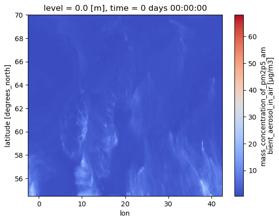
Plotting#
Plotting data can easily be obtained through matplotlib.pyplot back-end matplotlib documentation.
cams_AOI.isel(time=0).plot(cmap="coolwarm")
<matplotlib.collections.QuadMesh at 0x7f64f8af05c0>
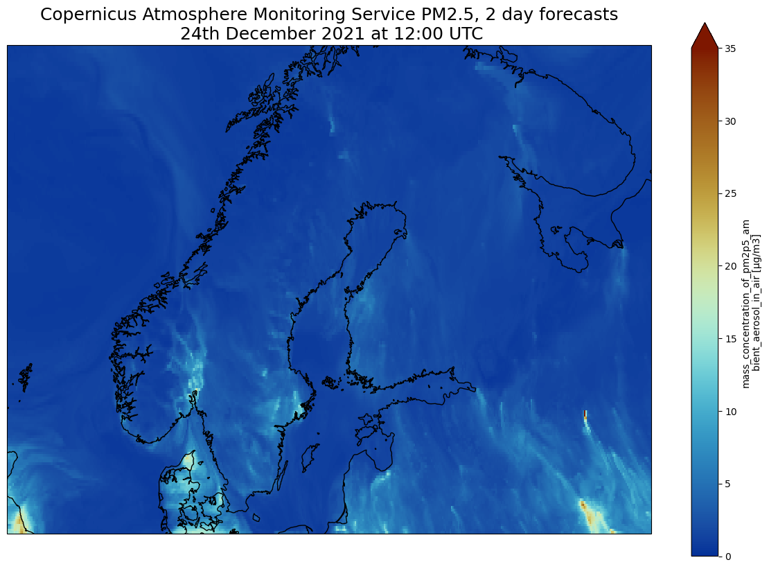
import matplotlib.pyplot as plt
import cartopy.crs as ccrs
import cmcrameri.cm as cmc
fig = plt.figure(1, figsize=[15,10])

# We're using cartopy to project our data.
# (see documentation on cartopy)
ax = plt.subplot(1, 1, 1, projection=ccrs.Mercator())
ax.coastlines(resolution='10m')

# We need to project our data to the new projection and for this we use `transform`.
# we set the original data projection in transform (here PlateCarree)
cams_AOI.isel(time=0).plot(ax=ax,
                                                                                    transform=ccrs.PlateCarree(),
                                                                                    vmin = 0, vmax = 35,
                                                                                    cmap=cmc.roma_r)
# One way to customize your title
plt.title("Copernicus Atmosphere Monitoring Service PM2.5, 2 day forecasts\n 24th December 2021 at 12:00 UTC", fontsize=18)
plt.savefig("CAMS-PM2_5-fc-20211224.png")
In the next episode, we will learn more about advanced visualization tools and how to make interactive plots using holoviews, a tool part of the HoloViz ecosystem.
Basic maths#
PM2.5 values are in µg/m3 and we can easily convert them in ng/m3 by multiplying the values by 1000.
Simple arithmetic operations can be performed without worrying about dimensions and coordinates, using the same notation we use with numpy. Underneath xarray will automatically vectorize the operations over all the data dimensions.
cams_AOI*1000
<xarray.DataArray 'pm2p5_conc' (time: 97, level: 1, lat: 155, lon: 450)> Size: 27MB
array([[[[  855.6641 ,   852.48096,   833.32465, ...,   879.8937 ,
            902.90106,   865.896  ],
         [  885.7343 ,   891.02075,   878.97   , ...,   971.65314,
           1061.4657 ,  1015.5647 ],
         [  893.89136,   828.7204 ,   800.25604, ...,  1032.3335 ,
            990.852  ,   982.55286],
         ...,
         [10043.194  , 10672.565  , 11238.228  , ...,  7507.282  ,
           7414.5137 ,  7444.7827 ],
         [13826.692  , 14108.494  , 14563.739  , ...,  7519.0063 ,
           7214.311  ,  7085.4043 ],
         [14878.069  , 14873.55   , 14858.358  , ...,  7069.7866 ,
           7237.475  ,  7302.5605 ]]],


       [[[  868.89185,   899.5873 ,   930.3964 , ...,   936.80554,
            839.1485 ,   772.7412 ],
         [  858.319  ,   891.28815,   934.2618 , ...,   772.7412 ,
            733.67554,   716.23883],
         [  873.09827,   925.96265,   940.6993 , ...,   729.8386 ,
...
           6790.51   ,  6748.986  ],
         [ 1623.8978 ,  1855.4778 ,  2173.332  , ...,  5969.662  ,
           6049.47   ,  6131.5386 ],
         [ 2051.7156 ,  2147.7383 ,  1941.084  , ...,  5981.9263 ,
           5846.8096 ,  5826.9146 ]]],


       [[[ 1362.0598 ,  1371.5527 ,  1349.8243 , ...,  2480.518  ,
           2496.761  ,  2526.6606 ],
         [ 1398.2976 ,  1351.3591 ,  1315.5477 , ...,  2294.1143 ,
           2327.9363 ,  2370.2136 ],
         [ 1287.1544 ,  1304.108  ,  1268.4387 , ...,  2281.4312 ,
           2239.3528 ,  2212.153  ],
         ...,
         [ 1829.8173 ,  1892.3165 ,  1997.889  , ...,  6986.432  ,
           6914.4253 ,  6935.685  ],
         [ 1650.3838 ,  1853.0875 ,  2025.124  , ...,  6504.3003 ,
           6350.027  ,  6176.655  ],
         [ 1954.8159 ,  2019.9797 ,  1916.7521 , ...,  5647.4995 ,
           5836.5464 ,  6040.9556 ]]]], dtype=float32)
Coordinates:
  * lat      (lat) float32 620B 69.95 69.85 69.75 69.65 ... 54.75 54.65 54.55
  * level    (level) float32 4B 0.0
  * time     (time) timedelta64[ns] 776B 00:00:00 01:00:00 ... 4 days 00:00:00
* lon (lon) float32 2kB -2.45 -2.35 -2.25 -2.15 ... 42.25 42.35 42.45The universal function (ufunc) from numpy and scipy can be applied too directly to the data. There are currently more than 60 universal functions defined in numpy on one or more types, covering a wide variety of operations including math operations, trigonometric functions, etc.
np.multiply(cams_AOI, 1000)
<xarray.DataArray 'pm2p5_conc' (time: 97, level: 1, lat: 155, lon: 450)> Size: 27MB
array([[[[  855.6641 ,   852.48096,   833.32465, ...,   879.8937 ,
            902.90106,   865.896  ],
         [  885.7343 ,   891.02075,   878.97   , ...,   971.65314,
           1061.4657 ,  1015.5647 ],
         [  893.89136,   828.7204 ,   800.25604, ...,  1032.3335 ,
            990.852  ,   982.55286],
         ...,
         [10043.194  , 10672.565  , 11238.228  , ...,  7507.282  ,
           7414.5137 ,  7444.7827 ],
         [13826.692  , 14108.494  , 14563.739  , ...,  7519.0063 ,
           7214.311  ,  7085.4043 ],
         [14878.069  , 14873.55   , 14858.358  , ...,  7069.7866 ,
           7237.475  ,  7302.5605 ]]],


       [[[  868.89185,   899.5873 ,   930.3964 , ...,   936.80554,
            839.1485 ,   772.7412 ],
         [  858.319  ,   891.28815,   934.2618 , ...,   772.7412 ,
            733.67554,   716.23883],
         [  873.09827,   925.96265,   940.6993 , ...,   729.8386 ,
...
           6790.51   ,  6748.986  ],
         [ 1623.8978 ,  1855.4778 ,  2173.332  , ...,  5969.662  ,
           6049.47   ,  6131.5386 ],
         [ 2051.7156 ,  2147.7383 ,  1941.084  , ...,  5981.9263 ,
           5846.8096 ,  5826.9146 ]]],


       [[[ 1362.0598 ,  1371.5527 ,  1349.8243 , ...,  2480.518  ,
           2496.761  ,  2526.6606 ],
         [ 1398.2976 ,  1351.3591 ,  1315.5477 , ...,  2294.1143 ,
           2327.9363 ,  2370.2136 ],
         [ 1287.1544 ,  1304.108  ,  1268.4387 , ...,  2281.4312 ,
           2239.3528 ,  2212.153  ],
         ...,
         [ 1829.8173 ,  1892.3165 ,  1997.889  , ...,  6986.432  ,
           6914.4253 ,  6935.685  ],
         [ 1650.3838 ,  1853.0875 ,  2025.124  , ...,  6504.3003 ,
           6350.027  ,  6176.655  ],
         [ 1954.8159 ,  2019.9797 ,  1916.7521 , ...,  5647.4995 ,
           5836.5464 ,  6040.9556 ]]]], dtype=float32)
Coordinates:
* lat (lat) float32 620B 69.95 69.85 69.75 69.65 ... 54.75 54.65 54.55
* level (level) float32 4B 0.0
* time (time) timedelta64[ns] 776B 00:00:00 01:00:00 ... 4 days 00:00:00
* lon (lon) float32 2kB -2.45 -2.35 -2.25 -2.15 ... 42.25 42.35 42.45
Attributes:
species: PM2.5 Aerosol
units: µg/m3
value: hourly values
standard_name: mass_concentration_of_pm2p5_ambient_aerosol_in_aircams_AOI = cams_AOI * 1000
cams_AOI
<xarray.DataArray 'pm2p5_conc' (time: 97, level: 1, lat: 155, lon: 450)> Size: 27MB
array([[[[ 855.6641 , 852.48096, 833.32465, ..., 879.8937 ,
902.90106, 865.896 ],
[ 885.7343 , 891.02075, 878.97 , ..., 971.65314,
1061.4657 , 1015.5647 ],
[ 893.89136, 828.7204 , 800.25604, ..., 1032.3335 ,
990.852 , 982.55286],
...,
[10043.194 , 10672.565 , 11238.228 , ..., 7507.282 ,
7414.5137 , 7444.7827 ],
[13826.692 , 14108.494 , 14563.739 , ..., 7519.0063 ,
7214.311 , 7085.4043 ],
[14878.069 , 14873.55 , 14858.358 , ..., 7069.7866 ,
7237.475 , 7302.5605 ]]],
[[[ 868.89185, 899.5873 , 930.3964 , ..., 936.80554,
839.1485 , 772.7412 ],
[ 858.319 , 891.28815, 934.2618 , ..., 772.7412 ,
733.67554, 716.23883],
[ 873.09827, 925.96265, 940.6993 , ..., 729.8386 ,
...
6790.51 , 6748.986 ],
[ 1623.8978 , 1855.4778 , 2173.332 , ..., 5969.662 ,
6049.47 , 6131.5386 ],
[ 2051.7156 , 2147.7383 , 1941.084 , ..., 5981.9263 ,
5846.8096 , 5826.9146 ]]],
[[[ 1362.0598 , 1371.5527 , 1349.8243 , ..., 2480.518 ,
2496.761 , 2526.6606 ],
[ 1398.2976 , 1351.3591 , 1315.5477 , ..., 2294.1143 ,
2327.9363 , 2370.2136 ],
[ 1287.1544 , 1304.108 , 1268.4387 , ..., 2281.4312 ,
2239.3528 , 2212.153 ],
...,
[ 1829.8173 , 1892.3165 , 1997.889 , ..., 6986.432 ,
6914.4253 , 6935.685 ],
[ 1650.3838 , 1853.0875 , 2025.124 , ..., 6504.3003 ,
6350.027 , 6176.655 ],
[ 1954.8159 , 2019.9797 , 1916.7521 , ..., 5647.4995 ,
5836.5464 , 6040.9556 ]]]], dtype=float32)
Coordinates:
* lat (lat) float32 620B 69.95 69.85 69.75 69.65 ... 54.75 54.65 54.55
* level (level) float32 4B 0.0
* time (time) timedelta64[ns] 776B 00:00:00 01:00:00 ... 4 days 00:00:00
* lon (lon) float32 2kB -2.45 -2.35 -2.25 -2.15 ... 42.25 42.35 42.45Updating attributes#
As we changed the units of the variable PM2.5, we need to reflect this change in the metadata of the data e.g. the attributes of pm2p5_conc. As we can see above, the operation did not keep any attributes so we will first copy the attributes from the original dataset and update the units.
cams_AOI.attrs = cams.pm2p5_conc.attrs
cams_AOI
<xarray.DataArray 'pm2p5_conc' (time: 97, level: 1, lat: 155, lon: 450)> Size: 27MB
array([[[[  855.6641 ,   852.48096,   833.32465, ...,   879.8937 ,
            902.90106,   865.896  ],
         [  885.7343 ,   891.02075,   878.97   , ...,   971.65314,
           1061.4657 ,  1015.5647 ],
         [  893.89136,   828.7204 ,   800.25604, ...,  1032.3335 ,
            990.852  ,   982.55286],
         ...,
         [10043.194  , 10672.565  , 11238.228  , ...,  7507.282  ,
           7414.5137 ,  7444.7827 ],
         [13826.692  , 14108.494  , 14563.739  , ...,  7519.0063 ,
           7214.311  ,  7085.4043 ],
         [14878.069  , 14873.55   , 14858.358  , ...,  7069.7866 ,
           7237.475  ,  7302.5605 ]]],


       [[[  868.89185,   899.5873 ,   930.3964 , ...,   936.80554,
            839.1485 ,   772.7412 ],
         [  858.319  ,   891.28815,   934.2618 , ...,   772.7412 ,
            733.67554,   716.23883],
         [  873.09827,   925.96265,   940.6993 , ...,   729.8386 ,
...
           6790.51   ,  6748.986  ],
         [ 1623.8978 ,  1855.4778 ,  2173.332  , ...,  5969.662  ,
           6049.47   ,  6131.5386 ],
         [ 2051.7156 ,  2147.7383 ,  1941.084  , ...,  5981.9263 ,
           5846.8096 ,  5826.9146 ]]],


       [[[ 1362.0598 ,  1371.5527 ,  1349.8243 , ...,  2480.518  ,
           2496.761  ,  2526.6606 ],
         [ 1398.2976 ,  1351.3591 ,  1315.5477 , ...,  2294.1143 ,
           2327.9363 ,  2370.2136 ],
         [ 1287.1544 ,  1304.108  ,  1268.4387 , ...,  2281.4312 ,
           2239.3528 ,  2212.153  ],
         ...,
         [ 1829.8173 ,  1892.3165 ,  1997.889  , ...,  6986.432  ,
           6914.4253 ,  6935.685  ],
         [ 1650.3838 ,  1853.0875 ,  2025.124  , ...,  6504.3003 ,
           6350.027  ,  6176.655  ],
         [ 1954.8159 ,  2019.9797 ,  1916.7521 , ...,  5647.4995 ,
           5836.5464 ,  6040.9556 ]]]], dtype=float32)
Coordinates:
  * lat      (lat) float32 620B 69.95 69.85 69.75 69.65 ... 54.75 54.65 54.55
  * level    (level) float32 4B 0.0
  * time     (time) timedelta64[ns] 776B 00:00:00 01:00:00 ... 4 days 00:00:00
  * lon      (lon) float32 2kB -2.45 -2.35 -2.25 -2.15 ... 42.25 42.35 42.45
Attributes:
    species:        PM2.5 Aerosol
    units:          µg/m3
    value:          hourly values
standard_name: mass_concentration_of_pm2p5_ambient_aerosol_in_aircams_AOI.attrs["units"] = "ng/m3"
cams_AOI
<xarray.DataArray 'pm2p5_conc' (time: 97, level: 1, lat: 155, lon: 450)> Size: 27MB
array([[[[  855.6641 ,   852.48096,   833.32465, ...,   879.8937 ,
            902.90106,   865.896  ],
         [  885.7343 ,   891.02075,   878.97   , ...,   971.65314,
           1061.4657 ,  1015.5647 ],
         [  893.89136,   828.7204 ,   800.25604, ...,  1032.3335 ,
            990.852  ,   982.55286],
         ...,
         [10043.194  , 10672.565  , 11238.228  , ...,  7507.282  ,
           7414.5137 ,  7444.7827 ],
         [13826.692  , 14108.494  , 14563.739  , ...,  7519.0063 ,
           7214.311  ,  7085.4043 ],
         [14878.069  , 14873.55   , 14858.358  , ...,  7069.7866 ,
           7237.475  ,  7302.5605 ]]],


       [[[  868.89185,   899.5873 ,   930.3964 , ...,   936.80554,
            839.1485 ,   772.7412 ],
         [  858.319  ,   891.28815,   934.2618 , ...,   772.7412 ,
            733.67554,   716.23883],
         [  873.09827,   925.96265,   940.6993 , ...,   729.8386 ,
...
           6790.51   ,  6748.986  ],
         [ 1623.8978 ,  1855.4778 ,  2173.332  , ...,  5969.662  ,
           6049.47   ,  6131.5386 ],
         [ 2051.7156 ,  2147.7383 ,  1941.084  , ...,  5981.9263 ,
           5846.8096 ,  5826.9146 ]]],


       [[[ 1362.0598 ,  1371.5527 ,  1349.8243 , ...,  2480.518  ,
           2496.761  ,  2526.6606 ],
         [ 1398.2976 ,  1351.3591 ,  1315.5477 , ...,  2294.1143 ,
           2327.9363 ,  2370.2136 ],
         [ 1287.1544 ,  1304.108  ,  1268.4387 , ...,  2281.4312 ,
           2239.3528 ,  2212.153  ],
         ...,
         [ 1829.8173 ,  1892.3165 ,  1997.889  , ...,  6986.432  ,
           6914.4253 ,  6935.685  ],
         [ 1650.3838 ,  1853.0875 ,  2025.124  , ...,  6504.3003 ,
           6350.027  ,  6176.655  ],
         [ 1954.8159 ,  2019.9797 ,  1916.7521 , ...,  5647.4995 ,
           5836.5464 ,  6040.9556 ]]]], dtype=float32)
Coordinates:
* lat (lat) float32 620B 69.95 69.85 69.75 69.65 ... 54.75 54.65 54.55
* level (level) float32 4B 0.0
* time (time) timedelta64[ns] 776B 00:00:00 01:00:00 ... 4 days 00:00:00
* lon (lon) float32 2kB -2.45 -2.35 -2.25 -2.15 ... 42.25 42.35 42.45
Attributes:
species: PM2.5 Aerosol
units: ng/m3
value: hourly values
standard_name: mass_concentration_of_pm2p5_ambient_aerosol_in_airStatistics#
All the standard statistical operations can be used such as min, max, mean. When no argument is passed to the function, the operation is done over all the dimensions of the variable (same as with numpy).
cams_AOI.min()
<xarray.DataArray 'pm2p5_conc' ()> Size: 4B array(375.9604, dtype=float32)
You can make a statistical operation over a dimension. For instance, let’s retrieve the maximum pm2p5_conc value among all those available for different times, at each lat-lon location.
cams_AOI.max(dim='time')
<xarray.DataArray 'pm2p5_conc' (level: 1, lat: 155, lon: 450)> Size: 279kB
array([[[ 2121.0813, 2219.4773, 2217.5305, ..., 3652.913 ,
3473.7568, 3577.1978],
[ 2229.2544, 2233.2195, 2240.6362, ..., 4046.014 ,
3602.7063, 3208.9517],
[ 2284.292 , 2295.2058, 2309.7578, ..., 4741.6777,
4632.1265, 4161.8325],
...,
[13408.843 , 13095.977 , 14038.214 , ..., 18508.65 ,
18356.64 , 17824.658 ],
[17083.7 , 16497.771 , 16912.217 , ..., 19211.908 ,
19491.762 , 18477.52 ],
[19680.336 , 19178.678 , 18560.22 , ..., 18558.336 ,
18246.791 , 18232.215 ]]], dtype=float32)
Coordinates:
* lat (lat) float32 620B 69.95 69.85 69.75 69.65 ... 54.75 54.65 54.55
* level (level) float32 4B 0.0
* lon (lon) float32 2kB -2.45 -2.35 -2.25 -2.15 ... 42.25 42.35 42.45Aggregation#
We have hourly data. To obtain daily values, we can group values per day and compute the mean. Let’s first convert the time in a more human readable manner.
import pandas as pd
list_times = np.datetime64('2021-12-22') + cams.time
print(pd.to_datetime(list_times).strftime("%d %b %H:%S UTC"))
Index(['22 Dec 00:00 UTC', '22 Dec 01:00 UTC', '22 Dec 02:00 UTC',
'22 Dec 03:00 UTC', '22 Dec 04:00 UTC', '22 Dec 05:00 UTC',
'22 Dec 06:00 UTC', '22 Dec 07:00 UTC', '22 Dec 08:00 UTC',
'22 Dec 09:00 UTC', '22 Dec 10:00 UTC', '22 Dec 11:00 UTC',
'22 Dec 12:00 UTC', '22 Dec 13:00 UTC', '22 Dec 14:00 UTC',
'22 Dec 15:00 UTC', '22 Dec 16:00 UTC', '22 Dec 17:00 UTC',
'22 Dec 18:00 UTC', '22 Dec 19:00 UTC', '22 Dec 20:00 UTC',
'22 Dec 21:00 UTC', '22 Dec 22:00 UTC', '22 Dec 23:00 UTC',
'23 Dec 00:00 UTC', '23 Dec 01:00 UTC', '23 Dec 02:00 UTC',
'23 Dec 03:00 UTC', '23 Dec 04:00 UTC', '23 Dec 05:00 UTC',
'23 Dec 06:00 UTC', '23 Dec 07:00 UTC', '23 Dec 08:00 UTC',
'23 Dec 09:00 UTC', '23 Dec 10:00 UTC', '23 Dec 11:00 UTC',
'23 Dec 12:00 UTC', '23 Dec 13:00 UTC', '23 Dec 14:00 UTC',
'23 Dec 15:00 UTC', '23 Dec 16:00 UTC', '23 Dec 17:00 UTC',
'23 Dec 18:00 UTC', '23 Dec 19:00 UTC', '23 Dec 20:00 UTC',
'23 Dec 21:00 UTC', '23 Dec 22:00 UTC', '23 Dec 23:00 UTC',
'24 Dec 00:00 UTC', '24 Dec 01:00 UTC', '24 Dec 02:00 UTC',
'24 Dec 03:00 UTC', '24 Dec 04:00 UTC', '24 Dec 05:00 UTC',
'24 Dec 06:00 UTC', '24 Dec 07:00 UTC', '24 Dec 08:00 UTC',
'24 Dec 09:00 UTC', '24 Dec 10:00 UTC', '24 Dec 11:00 UTC',
'24 Dec 12:00 UTC', '24 Dec 13:00 UTC', '24 Dec 14:00 UTC',
'24 Dec 15:00 UTC', '24 Dec 16:00 UTC', '24 Dec 17:00 UTC',
'24 Dec 18:00 UTC', '24 Dec 19:00 UTC', '24 Dec 20:00 UTC',
'24 Dec 21:00 UTC', '24 Dec 22:00 UTC', '24 Dec 23:00 UTC',
'25 Dec 00:00 UTC', '25 Dec 01:00 UTC', '25 Dec 02:00 UTC',
'25 Dec 03:00 UTC', '25 Dec 04:00 UTC', '25 Dec 05:00 UTC',
'25 Dec 06:00 UTC', '25 Dec 07:00 UTC', '25 Dec 08:00 UTC',
'25 Dec 09:00 UTC', '25 Dec 10:00 UTC', '25 Dec 11:00 UTC',
'25 Dec 12:00 UTC', '25 Dec 13:00 UTC', '25 Dec 14:00 UTC',
'25 Dec 15:00 UTC', '25 Dec 16:00 UTC', '25 Dec 17:00 UTC',
'25 Dec 18:00 UTC', '25 Dec 19:00 UTC', '25 Dec 20:00 UTC',
'25 Dec 21:00 UTC', '25 Dec 22:00 UTC', '25 Dec 23:00 UTC',
'26 Dec 00:00 UTC'],
dtype='object')
cams_AOI["time"] = list_times
cams_AOI
<xarray.DataArray 'pm2p5_conc' (time: 97, level: 1, lat: 155, lon: 450)> Size: 27MB
array([[[[  855.6641 ,   852.48096,   833.32465, ...,   879.8937 ,
            902.90106,   865.896  ],
         [  885.7343 ,   891.02075,   878.97   , ...,   971.65314,
           1061.4657 ,  1015.5647 ],
         [  893.89136,   828.7204 ,   800.25604, ...,  1032.3335 ,
            990.852  ,   982.55286],
         ...,
         [10043.194  , 10672.565  , 11238.228  , ...,  7507.282  ,
           7414.5137 ,  7444.7827 ],
         [13826.692  , 14108.494  , 14563.739  , ...,  7519.0063 ,
           7214.311  ,  7085.4043 ],
         [14878.069  , 14873.55   , 14858.358  , ...,  7069.7866 ,
           7237.475  ,  7302.5605 ]]],


       [[[  868.89185,   899.5873 ,   930.3964 , ...,   936.80554,
            839.1485 ,   772.7412 ],
         [  858.319  ,   891.28815,   934.2618 , ...,   772.7412 ,
            733.67554,   716.23883],
         [  873.09827,   925.96265,   940.6993 , ...,   729.8386 ,
...
           6790.51   ,  6748.986  ],
         [ 1623.8978 ,  1855.4778 ,  2173.332  , ...,  5969.662  ,
           6049.47   ,  6131.5386 ],
         [ 2051.7156 ,  2147.7383 ,  1941.084  , ...,  5981.9263 ,
           5846.8096 ,  5826.9146 ]]],


       [[[ 1362.0598 ,  1371.5527 ,  1349.8243 , ...,  2480.518  ,
           2496.761  ,  2526.6606 ],
         [ 1398.2976 ,  1351.3591 ,  1315.5477 , ...,  2294.1143 ,
           2327.9363 ,  2370.2136 ],
         [ 1287.1544 ,  1304.108  ,  1268.4387 , ...,  2281.4312 ,
           2239.3528 ,  2212.153  ],
         ...,
         [ 1829.8173 ,  1892.3165 ,  1997.889  , ...,  6986.432  ,
           6914.4253 ,  6935.685  ],
         [ 1650.3838 ,  1853.0875 ,  2025.124  , ...,  6504.3003 ,
           6350.027  ,  6176.655  ],
         [ 1954.8159 ,  2019.9797 ,  1916.7521 , ...,  5647.4995 ,
           5836.5464 ,  6040.9556 ]]]], dtype=float32)
Coordinates:
* lat (lat) float32 620B 69.95 69.85 69.75 69.65 ... 54.75 54.65 54.55
* level (level) float32 4B 0.0
* lon (lon) float32 2kB -2.45 -2.35 -2.25 -2.15 ... 42.25 42.35 42.45
* time (time) datetime64[ns] 776B 2021-12-22 ... 2021-12-26
Attributes:
species: PM2.5 Aerosol
units: ng/m3
value: hourly values
standard_name: mass_concentration_of_pm2p5_ambient_aerosol_in_aircams_daily = cams_AOI.groupby(cams_AOI.time.dt.day).mean()
cams_daily
<xarray.DataArray 'pm2p5_conc' (day: 5, level: 1, lat: 155, lon: 450)> Size: 1MB
array([[[[ 1169.239  ,  1166.6467 ,  1160.973  , ...,  1441.5961 ,
           1446.9415 ,  1449.0151 ],
         [ 1173.6224 ,  1171.9554 ,  1171.7555 , ...,  1428.3876 ,
           1443.7915 ,  1446.5171 ],
         [ 1181.1288 ,  1189.5563 ,  1205.5222 , ...,  1435.0128 ,
           1436.0138 ,  1443.3612 ],
         ...,
         [ 9959.0625 ,  9706.599  , 10212.829  , ...,  8834.37   ,
           8843.07   ,  8738.081  ],
         [11996.876  , 11674.386  , 11926.778  , ...,  8548.44   ,
           8362.801  ,  8002.9683 ],
         [13141.722  , 12680.837  , 12554.7    , ...,  7965.3184 ,
           7982.112  ,  7990.6177 ]]],


       [[[ 1686.1406 ,  1708.1188 ,  1722.3102 , ...,  1365.6635 ,
           1362.4203 ,  1382.3403 ],
         [ 1709.118  ,  1726.6967 ,  1740.0448 , ...,  1310.9231 ,
           1319.0963 ,  1326.693  ],
         [ 1732.6241 ,  1738.5929 ,  1748.2808 , ...,  1290.9888 ,
...
           4905.723  ,  4991.6763 ],
         [ 1478.167  ,  1535.4425 ,  1637.3916 , ...,  4755.4307 ,
           4620.1465 ,  4505.0903 ],
         [ 1717.3419 ,  1729.2365 ,  1662.1465 , ...,  4393.5034 ,
           4420.8423 ,  4419.639  ]]],


       [[[ 1362.0598 ,  1371.5527 ,  1349.8243 , ...,  2480.518  ,
           2496.761  ,  2526.6606 ],
         [ 1398.2976 ,  1351.3591 ,  1315.5477 , ...,  2294.1143 ,
           2327.9363 ,  2370.2136 ],
         [ 1287.1544 ,  1304.108  ,  1268.4387 , ...,  2281.4312 ,
           2239.3528 ,  2212.153  ],
         ...,
         [ 1829.8173 ,  1892.3165 ,  1997.889  , ...,  6986.432  ,
           6914.4253 ,  6935.685  ],
         [ 1650.3838 ,  1853.0875 ,  2025.124  , ...,  6504.3003 ,
           6350.027  ,  6176.655  ],
         [ 1954.8159 ,  2019.9797 ,  1916.7521 , ...,  5647.4995 ,
           5836.5464 ,  6040.9556 ]]]], dtype=float32)
Coordinates:
  * lat      (lat) float32 620B 69.95 69.85 69.75 69.65 ... 54.75 54.65 54.55
  * level    (level) float32 4B 0.0
  * lon      (lon) float32 2kB -2.45 -2.35 -2.25 -2.15 ... 42.25 42.35 42.45
  * day      (day) int64 40B 22 23 24 25 26
Attributes:
    species:        PM2.5 Aerosol
    units:          ng/m3
    value:          hourly values
standard_name: mass_concentration_of_pm2p5_ambient_aerosol_in_airAs we have data from 2021-12-22 to 2021-12-26, the time dimension is now day and takes values from 22 to 26.
cams_daily.day
<xarray.DataArray 'day' (day: 5)> Size: 40B
array([22, 23, 24, 25, 26])
Coordinates:
  * day      (day) int64 40B 22 23 24 25 26
Attributes:
long_name: FORECAST time from 20211222- Could you change the attribute "value" from "hourly values" to "daily values"?
Mask#
Masking can be achieved through the method DataSet|Array.where(cond, other) or xr.where(cond, x, y).
The difference consists in the possibility to specify the value in case the condition is positive or not; DataSet|Array.where(cond, other) only offer the possibility to define the false condition value (by default is set to np.NaN))
cams_AOI.min(), cams_AOI.max()
(<xarray.DataArray 'pm2p5_conc' ()> Size: 4B
 array(375.9604, dtype=float32),
 <xarray.DataArray 'pm2p5_conc' ()> Size: 4B
 array(86237.35, dtype=float32))
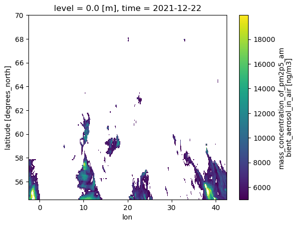
cams_masked = cams_AOI.where((cams_AOI >= 5000) & (cams_AOI <= 20000))
cams_masked.isel(time=0).plot()
<matplotlib.collections.QuadMesh at 0x7f64ed6f3ce0>
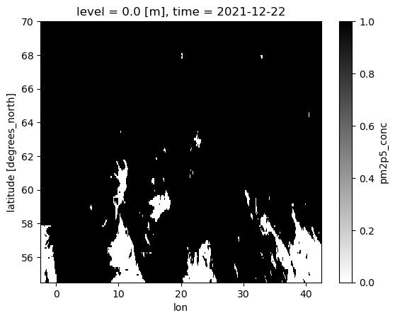
To better visualize the mask, with the help of xr.where, ad-hoc variables can be created. ‘xr.where’ lets us specify values of 1 for masked and 0 for the unmasked data.
mask = xr.where((cams_AOI <= 5000) | (cams_AOI >= 20000), 1, 0)
mask.isel(time=0).plot(cmap="binary")
<matplotlib.collections.QuadMesh at 0x7f64ed6f3f50>
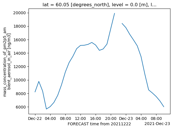
Plot a single point (defined by its latitude and longitude) over the time dimension.
cams_masked.sel(lat=60., lon=10.75, method='nearest').plot()
[<matplotlib.lines.Line2D at 0x7f64ed6f34a0>]
Save xarray Dataset#
It is very often convenient to save intermediate or final results into a local file. We will learn more about the different file formats Xarray can handle, but for now let’s save it as a netCDF file. Check the file size after saving the result into netCDF.
cams_masked.to_netcdf('cams_Nordic_masked.nc')
Advanced Saving methods#
Encoding and Compression#
From the near-surface temperature dataset we already know that values are encoded as float32. A compression method can be defined as well; if the format is netCDF4 with the engine set to ‘netcdf4’ or ‘h5netcdf’ there are different compression options. The easiest solution is to stick with the default one for NetCDF4 files.
Note that encoding parameters needs to be done through a nested dictionary and parameters have to be defined for each single variable.
cams_masked.to_netcdf('cams_Nordic_mcs.nc',
                      engine='netcdf4',
                      encoding={'pm2p5_conc':{"dtype": np.float32,
                                        'zlib': True, 'complevel':4}
                                }
                      )
- Xarray Dataset and DataArray
- Read and get metadata from local raster file
- Dataset and DataArray selection
- Aggregation and statistics
- Masking values
Through the datatype and the compression a compression of almost 10 time has been achieved; as drawback reading speed has been decreased.
References#
F.N. Kogan. Application of vegetation index and brightness temperature for drought detection. Advances in Space Research, 15(11):91–100, 1995. Natural Hazards: Monitoring and Assessment Using Remote Sensing Technique. URL: https://www.sciencedirect.com/science/article/pii/027311779500079T, doi:https://doi.org/10.1016/0273-1177(95)00079-T.
Wikipedia. Normalized difference vegetation index. https://en.wikipedia.org/wiki/Normalized_difference_vegetation_index, 2022 (accessed August 7, 2022).
Packages citation#
Fabio Crameri. Scientific colour maps. 2023. URL: https://zenodo.org/record/1243862, doi:10.5281/ZENODO.1243862.
Charles R. Harris, K. Jarrod Millman, Stéfan J. van der Walt, Ralf Gommers, Pauli Virtanen, David Cournapeau, Eric Wieser, Julian Taylor, Sebastian Berg, Nathaniel J. Smith, Robert Kern, Matti Picus, Stephan Hoyer, Marten H. van Kerkwijk, Matthew Brett, Allan Haldane, Jaime Fernández del Río, Mark Wiebe, Pearu Peterson, Pierre Gérard-Marchant, Kevin Sheppard, Tyler Reddy, Warren Weckesser, Hameer Abbasi, Christoph Gohlke, and Travis E. Oliphant. Array programming with NumPy. Nature, 585(7825):357–362, September 2020. URL: https://doi.org/10.1038/s41586-020-2649-2, doi:10.1038/s41586-020-2649-2.
S. Hoyer and J. Hamman. Xarray: N-D labeled arrays and datasets in Python. Journal of Open Research Software, 2017. URL: https://doi.org/10.5334/jors.148, doi:10.5334/jors.148.
Leonardo Uieda, Santiago Rubén Soler, Rémi Rampin, Hugo van Kemenade, Matthew Turk, Daniel Shapero, Anderson Banihirwe, and John Leeman. Pooch: a friend to fetch your data files. Journal of Open Source Software, 5(45):1943, 2020. URL: https://doi.org/10.21105/joss.01943, doi:10.21105/joss.01943.