Global Earth Observation imagery and HEALPix#
Context#
Earth Observation images naturally represent data on a spheroidal surface. In this notebook, we introduce HEALPix, a powerful indexing scheme for organizing spheroidal data, together with the Zarr storage format. By combining these two technologies, we can analyze Earth Observation data in its native form.
Because remote sensing datasets can be quite large, we also use Dask with Xarray to parallelize our data analysis.
Data#
In this episode, we will be using datasets from Copernicus Marine Service:
ODYSSEA Global Sea Surface Temperature Gridded Level 4 Daily Multi-Sensor Observations. DOI (product): h10.48670/mds-00321)
The datasetst are probided in Zarr format and Netcdf format and will be accessed through S3-compatible object storage or Ifremer’s https server.
Setup#
This episode uses the following main Python packages:
Please install these packages if not already available in your Python environment.
Packages#
In this episode, Python packages are imported when we start to use them. However, for best software practices, we recommend you to install and import all the necessary libraries at the top of your Jupyter notebook.
Installation of required packages#
!pip install -U xdggs copernicusmarine healpix_geo healpy flox
Import necessary libraries#
import xarray as xr
import numpy as np
import fsspec
import pint_xarray
import cf_xarray.units
import healpy as hp
import matplotlib.pyplot as plt
import xdggs
import hvplot.xarray
import copernicusmarine
from copernicusmarine.core_functions import custom_open_zarr
from healpix_geo.nested import lonlat_to_healpix
Create a local Dask cluster on the local machine#
from dask.distributed import Client
client = Client() # create a local dask cluster on the local machine.
client
Client
Client-86e42ebe-9cf1-11f0-8144-5ef18bd36582
| Connection method: Cluster object | Cluster type: distributed.LocalCluster |
| Dashboard: http://127.0.0.1:8787/status |
Cluster Info
LocalCluster
a70882c4
| Dashboard: http://127.0.0.1:8787/status | Workers: 4 |
| Total threads: 8 | Total memory: 32.00 GiB |
| Status: running | Using processes: True |
Scheduler Info
Scheduler
Scheduler-ee8f10ea-19ec-49cf-9cd4-066f6f078eac
| Comm: tcp://127.0.0.1:38435 | Workers: 0 |
| Dashboard: http://127.0.0.1:8787/status | Total threads: 0 |
| Started: Just now | Total memory: 0 B |
Workers
Worker: 0
| Comm: tcp://127.0.0.1:45523 | Total threads: 2 |
| Dashboard: http://127.0.0.1:41053/status | Memory: 8.00 GiB |
| Nanny: tcp://127.0.0.1:46013 | |
| Local directory: /tmp/dask-scratch-space/worker-q9a9hcd5 | |
Worker: 1
| Comm: tcp://127.0.0.1:41481 | Total threads: 2 |
| Dashboard: http://127.0.0.1:35829/status | Memory: 8.00 GiB |
| Nanny: tcp://127.0.0.1:38633 | |
| Local directory: /tmp/dask-scratch-space/worker-0jlpohhx | |
Worker: 2
| Comm: tcp://127.0.0.1:46189 | Total threads: 2 |
| Dashboard: http://127.0.0.1:36989/status | Memory: 8.00 GiB |
| Nanny: tcp://127.0.0.1:41033 | |
| Local directory: /tmp/dask-scratch-space/worker-edp7sjti | |
Worker: 3
| Comm: tcp://127.0.0.1:38009 | Total threads: 2 |
| Dashboard: http://127.0.0.1:40945/status | Memory: 8.00 GiB |
| Nanny: tcp://127.0.0.1:34805 | |
| Local directory: /tmp/dask-scratch-space/worker-ron2ogyi | |
Inspecting the Cluster Info section above gives us information about the created cluster: we have 2 or 4 workers and the same number of threads (e.g. 1 thread per worker).
- You can also create a local cluster with the `LocalCluster` constructor and use `n_workers` and `threads_per_worker` to manually specify the number of processes and threads you want to use. For instance, we could use `n_workers=2` and `threads_per_worker=2`.
- This is sometimes preferable (in terms of performance), or when you run this tutorial on your PC, you can avoid dask to use all your resources you have on your PC!
Dask Dashboard#
Dask comes with a really handy interface: the Dask Dashboard. It is a web interface that you can open in a separate tab of your browser.
We will learn here how to use it through the Dask JupyterLab extension.
To use the Dask Dashboard through the JupyterLab extension on the Pangeo EOSC infrastructure, you will just need to click Launch dashboard in JupyterLab at the Client configuration in your JupyterLab, and the Dask dashboard port number, as highlighted in the figure below.
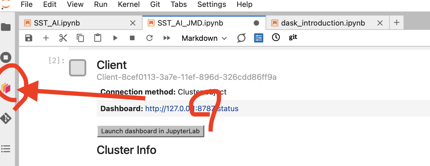
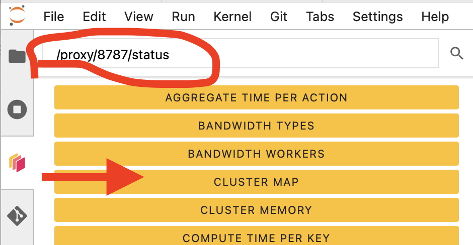
Then click the orange icon indicated in the above figure, and type your dashboard link.
You can click several buttons indicated with red arrows in the above figures, then drag and drop them to place them as per your convenience.
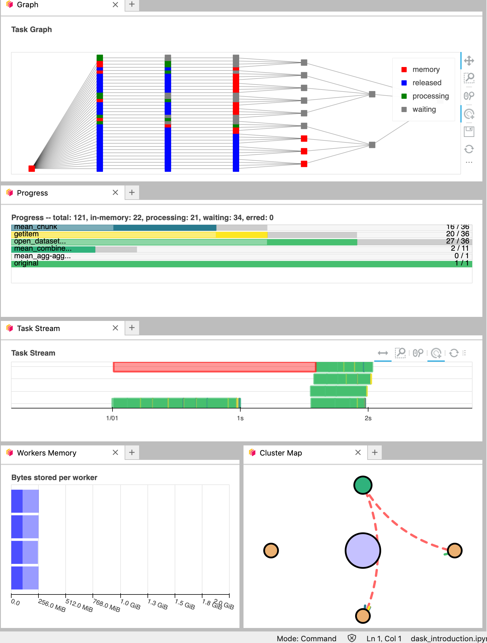
It’s really helpful to understand your computation and how it is distributed.
Data Loading: Get data from Copernicus Marine Services#
Data from Copernicus Marine Service is available in zarr format via s3-compatible object storage which make this data easily and efficiently accessible.
Lets choose the date we want to test.
time_slice = slice('2024-06-01', '2024-06-01')
Load L4 Dataset from Copernicus Marine Services#
This dataset provides a time series of gap-free maps of Sea Surface Temperature (SST) foundation at high resolution on a 0.10 x 0.10 degree grid (approximately 10 x 10 km) for the Global Ocean, updated every 24 hours.
We load the data in L4 and select one date.
Geo Chunk and Time Chunk#
Let’s try to load data in ‘geo’ chunked format and ‘time’ chunked format to see the differences.
url = "https://s3.waw3-1.cloudferro.com/mdl-arco-geo-045/arco/SST_GLO_PHY_L4_NRT_010_043/cmems_obs-sst_glo_phy_nrt_l4_P1D-m_202303/geoChunked.zarr"
url = "https://s3.waw3-1.cloudferro.com/mdl-arco-time-045/arco/SST_GLO_PHY_L4_NRT_010_043/cmems_obs-sst_glo_phy_nrt_l4_P1D-m_202303/timeChunked.zarr"
L4 = custom_open_zarr.open_zarr(url, )#**zarr_kwargs)
L4 = copernicusmarine.open_dataset( #dataset_id="cmems_obs-sst_glo_phy_l4_gir_P1D-m"
dataset_id="cmems_obs-sst_glo_phy_nrt_l4_P1D-m",)
L4=L4.sel(time=time_slice)
L4
INFO - 2025-09-29T04:26:40Z - Selected dataset version: "202303"
INFO - 2025-09-29T04:26:40Z - Selected dataset part: "default"
<xarray.Dataset> Size: 144MB
Dimensions: (time: 1, latitude: 1600, longitude: 3600)
Coordinates:
* latitude (latitude) float32 6kB -79.95 -79.85 ... 79.85 79.95
* longitude (longitude) float32 14kB -179.9 -179.9 ... 179.9 179.9
* time (time) datetime64[ns] 8B 2024-06-01
Data variables:
analysed_sst (time, latitude, longitude) float64 46MB dask.array<chunksize=(1, 64, 3200), meta=np.ndarray>
analysis_error (time, latitude, longitude) float64 46MB dask.array<chunksize=(1, 64, 3200), meta=np.ndarray>
mask (time, latitude, longitude) int8 6MB dask.array<chunksize=(1, 64, 3200), meta=np.ndarray>
sea_ice_fraction (time, latitude, longitude) float64 46MB dask.array<chunksize=(1, 64, 3200), meta=np.ndarray>
Attributes:
Conventions: CF-1.7, ACDD-1.3, ISO 8601
institution: Institut Francais de Recherche pour l'Exploitation de la me...
source: Odyssea L4 processor
references: Product User Manual for L4 Odyssea Product over the Global ...
contact: emmanuelle.autret@ifremer.fr;jfpiolle@ifremer.fr
title: ODYSSEA Global Sea Surface Temperature Gridded Level 4 Dail...
history: Optimally interpolated SST originally produced by Ifremer/C...%%time
url = 'https://data-cersat.ifremer.fr/data/sea-surface-temperature/odyssea/l4/glob/nrt/data/v3.0/2023/00*/*-IFR-L4_GHRSST-SSTfnd-ODYSSEA-GLOB_010-v02.1-fv01.0.nc'
# Create an HTTP filesystem
fs = fsspec.filesystem('http')
# Use fs.glob to expand the wildcard and get all matching files
file_list = fs.glob(url)
# Open the datasets with xarray
L4 = xr.open_mfdataset([fs.open(f) for f in file_list], engine='h5netcdf').chunk({"time":1, "lat":'auto', "lon":'10M'}).persist()
L4
CPU times: user 3.73 s, sys: 1.97 s, total: 5.7 s
Wall time: 59.6 s
<xarray.Dataset> Size: 1GB
Dimensions: (time: 9, lat: 1600, lon: 3600)
Coordinates:
* lat (lat) float32 6kB -79.95 -79.85 -79.75 ... 79.85 79.95
* lon (lon) float32 14kB -179.9 -179.9 -179.8 ... 179.9 179.9
* time (time) datetime64[ns] 72B 2023-01-01 ... 2023-01-09
Data variables:
analysed_sst (time, lat, lon) float64 415MB dask.array<chunksize=(1, 745, 1677), meta=np.ndarray>
analysis_error (time, lat, lon) float64 415MB dask.array<chunksize=(1, 745, 1677), meta=np.ndarray>
mask (time, lat, lon) int8 52MB dask.array<chunksize=(1, 1600, 3600), meta=np.ndarray>
sea_ice_fraction (time, lat, lon) float64 415MB dask.array<chunksize=(1, 745, 1677), meta=np.ndarray>
Attributes: (12/71)
Conventions: CF-1.7, ACDD-1.3, ISO 8601
standard_name_vocabulary: Climate and Forecast (CF) Standard Name ...
naming_authority: org.ghrsst
netcdf_version_id: 4.7.4 of Oct 31 2021 03:14:43 $
title: ODYSSEA Global Sea Surface Temperature G...
id: ODYSSEA-IFR-L4-GLOB_002-v3.0
... ...
doi: https://doi.org/10.48670/mds-00321
project: Copernicus Marine Service
program: Copernicus, GHRSST
publisher_name: Copernicus Marine Service
publisher_institution: Copernicus Marine Service
publisher_url: https://marine.copernicus.eu/- Where do you find attributes?
- What kind of data variables do you find in this dataset? What are the coordinates and dimensions?
- `geo` and `time`: which chunk is suitable for our computation??
Lets check the unit.#
L4['analysed_sst'].attrs
{'long_name': 'analysed sea surface temperature',
'standard_name': 'sea_surface_foundation_temperature',
'units': 'kelvin',
'valid_min': np.int16(-300),
'valid_max': np.int16(4500)}
L4['analysed_sst'].attrs['units']
'kelvin'
With pint xarray one can convert units. Lets convert SST L4 from Kelvin to Celcius.
L4['analysed_sst'].pint.quantify().pint.to("degC").pint.dequantify()
<xarray.DataArray 'analysed_sst' (time: 9, lat: 1600, lon: 3600)> Size: 415MB
dask.array<truediv, shape=(9, 1600, 3600), dtype=float64, chunksize=(1, 745, 1677), chunktype=numpy.ndarray>
Coordinates:
* lat (lat) float32 6kB -79.95 -79.85 -79.75 -79.65 ... 79.75 79.85 79.95
* lon (lon) float32 14kB -179.9 -179.9 -179.8 ... 179.8 179.9 179.9
* time (time) datetime64[ns] 72B 2023-01-01 2023-01-02 ... 2023-01-09
Attributes:
long_name: analysed sea surface temperature
standard_name: sea_surface_foundation_temperature
valid_min: -300
valid_max: 4500
units: degree_Celsiusds = L4[['analysed_sst']].pint.quantify().pint.to("degC").pint.dequantify()
ds
<xarray.Dataset> Size: 415MB
Dimensions: (time: 9, lat: 1600, lon: 3600)
Coordinates:
* lat (lat) float32 6kB -79.95 -79.85 -79.75 ... 79.75 79.85 79.95
* lon (lon) float32 14kB -179.9 -179.9 -179.8 ... 179.8 179.9 179.9
* time (time) datetime64[ns] 72B 2023-01-01 2023-01-02 ... 2023-01-09
Data variables:
analysed_sst (time, lat, lon) float64 415MB dask.array<chunksize=(1, 745, 1677), meta=np.ndarray>
Attributes: (12/71)
Conventions: CF-1.7, ACDD-1.3, ISO 8601
standard_name_vocabulary: Climate and Forecast (CF) Standard Name ...
naming_authority: org.ghrsst
netcdf_version_id: 4.7.4 of Oct 31 2021 03:14:43 $
title: ODYSSEA Global Sea Surface Temperature G...
id: ODYSSEA-IFR-L4-GLOB_002-v3.0
... ...
doi: https://doi.org/10.48670/mds-00321
project: Copernicus Marine Service
program: Copernicus, GHRSST
publisher_name: Copernicus Marine Service
publisher_institution: Copernicus Marine Service
publisher_url: https://marine.copernicus.eu/Lets try Persist() ;#
persist() load data from disk, triggers computation and keeps data as dask arrays in your memory.
Please watch carefully the dask lab view
ds=ds.persist()
ds
<xarray.Dataset> Size: 415MB
Dimensions: (time: 9, lat: 1600, lon: 3600)
Coordinates:
* lat (lat) float32 6kB -79.95 -79.85 -79.75 ... 79.75 79.85 79.95
* lon (lon) float32 14kB -179.9 -179.9 -179.8 ... 179.8 179.9 179.9
* time (time) datetime64[ns] 72B 2023-01-01 2023-01-02 ... 2023-01-09
Data variables:
analysed_sst (time, lat, lon) float64 415MB dask.array<chunksize=(1, 745, 1677), meta=np.ndarray>
Attributes: (12/71)
Conventions: CF-1.7, ACDD-1.3, ISO 8601
standard_name_vocabulary: Climate and Forecast (CF) Standard Name ...
naming_authority: org.ghrsst
netcdf_version_id: 4.7.4 of Oct 31 2021 03:14:43 $
title: ODYSSEA Global Sea Surface Temperature G...
id: ODYSSEA-IFR-L4-GLOB_002-v3.0
... ...
doi: https://doi.org/10.48670/mds-00321
project: Copernicus Marine Service
program: Copernicus, GHRSST
publisher_name: Copernicus Marine Service
publisher_institution: Copernicus Marine Service
publisher_url: https://marine.copernicus.eu/Save Dataset to local Zarr#
Zarr is a data format for storing chunked, compressed, N-dimensional arrays.
ds.to_zarr('SST.zarr', mode='w')
/srv/conda/envs/notebook/lib/python3.12/site-packages/zarr/api/asynchronous.py:228: UserWarning: Consolidated metadata is currently not part in the Zarr format 3 specification. It may not be supported by other zarr implementations and may change in the future.
warnings.warn(
<xarray.backends.zarr.ZarrStore at 0x739761578e00>
!ls
Bi-linear-plot.png agenda.md intro.md
SST.zarr assets landslide_xbatcher.ipynb
SST_AI.ipynb conf.py pangeo.md
Xbatcher_Sentinel2_wave.ipynb eo4eu_bids25.ipynb references.bib
_config.yml eosc-pangeo.md users-getting-started.md
_toc.yml healpix.zarr
afterword images
!ls -lart SST.zarr/analysed_sst/c/0
total 3
drwxr-xr-x 11 jovyan jovyan 4096 Sep 29 04:27 ..
drwxr-xr-x 5 jovyan jovyan 4096 Sep 29 04:27 .
drwxr-xr-x 2 jovyan jovyan 4096 Sep 29 04:27 0
drwxr-xr-x 2 jovyan jovyan 4096 Sep 29 04:28 2
drwxr-xr-x 2 jovyan jovyan 4096 Sep 29 04:28 1
!cat SST.zarr/zarr.json
{
"attributes": {
"Conventions": "CF-1.7, ACDD-1.3, ISO 8601",
"standard_name_vocabulary": "Climate and Forecast (CF) Standard Name Table v79",
"naming_authority": "org.ghrsst",
"netcdf_version_id": "4.7.4 of Oct 31 2021 03:14:43 $",
"title": "ODYSSEA Global Sea Surface Temperature Gridded Level 4 Daily Multi-Sensor Observations",
"id": "ODYSSEA-IFR-L4-GLOB_002-v3.0",
"cmems_product_id": "SST_GLO_PHY_L4_NRT_010_043",
"summary": "This dataset provide a times series of daily multi-sensor optimal interpolation of Sea Surface Temperature (SST) foundation over Global Ocean on a 0.1 degree resolution grid, every 24 hours. It is produced for the Copernicus Marine Service.",
"references": "Piolle J. F., Autret E., Arino O., Robinson I.S, Le Borgne P., (2010), Medspiration, toward the sustained delivery of satellite SST products and services over regional seas, Proceedings of the 2010 ESA Living Planet Symposium Bergen.",
"processing_level": "L4",
"keywords": "Oceans > Ocean Temperature > Sea Surface Temperature",
"keywords_vocabulary": "NASA Global Change Master Directory (GCMD) Science Keywords",
"institution": "Institut Francais de Recherche pour l'Exploitation de la mer / Centre d'Exploitation et de Recherche Satellitaire",
"institution_abbreviation": "Ifremer/CERSAT",
"license": "These data are available free of charge under the CMEMS data policy, refer to http://marine.copernicus.eu/services-portfolio/service-commitments-and-licence/",
"citation": "Ifremer / CERSAT. 2022. ODYSSEA Global High-Resolution Sea Surface Temperature Gridded Level 4 Daily dataset (v3.0) for Copernicus Marine Service. Ver. 3.0. Ifremer, Plouzane, France. Dataset accessed [YYYY-MM-DD].",
"contact": "emmanuelle.autret@ifremer.fr;jfpiolle@ifremer.fr",
"technical_support_contact": "cersat@ifremer.fr",
"scientific_support_contact": "emmanuelle.autret@ifremer.fr;jfpiolle@ifremer.fr",
"creator_email": "cersat@ifremer.fr",
"creator_type": "institution",
"creator_institution": "Ifremer / CERSAT",
"creator_name": "CERSAT",
"creator_url": "http://cersat.ifremer.fr",
"format_version": "GHRSST GDS v2.1",
"gds_version_id": "2.1",
"processing_software": "Odyssea 3.0",
"source": "Odyssea L4 processor",
"geospatial_bounds": "POLYGON ((-180.0 -80.0, 180.0 -80.0, 180.0 80.0, -180.0 80.0, -180.0 -80.0))",
"geospatial_bounds_crs": "EPSG:4326",
"geospatial_bounds_vertical_crs": "EPSG:5831",
"geospatial_lat_max": 80.0,
"geospatial_lat_min": -80.0,
"geospatial_lat_resolution": 0.1,
"geospatial_lat_units": "degrees_north",
"geospatial_lon_max": 180.0,
"geospatial_lon_min": -180.0,
"geospatial_lon_resolution": 0.1,
"geospatial_lon_units": "degrees_east",
"geospatial_vertical_min": 0.0,
"geospatial_vertical_max": 0.0,
"time_coverage_start": "2022-12-31T12:00:00",
"time_coverage_end": "2023-01-01T12:00:00",
"time_coverage_resolution": "P1D",
"spatial_resolution": "0.1 degree",
"temporal_resolution": "daily",
"cdm_data_type": "grid",
"source_data": "AVHRR_SST_METOP_B-OSISAF-L2P-v1.0 SLSTRA_MAR_L2P_v1.0 SLSTRB_MAR_L2P_v1.0 VIIRS_N20-STAR-L2P-v2.80 VIIRS_NPP-STAR-L2P-v2.80 GOES16-OSISAF-L3C-V1.0 G17-STAR-L3C-V2.71 SEVIRI_SST-OSISAF-L3C-V1.0 SEVIRI_IO_SST-OSISAF-L3C-V1.0 AHI_H08-STAR-L3C-v2.7 AMSR2-REMSS-L2P-v8.2",
"platform": "Metop-B Sentinel-3A Sentinel-3B NOAA-20 NPP GOES16 GOES17 Meteosat-11 Meteosat-9 Himawari-8 GCOM-W",
"platform_type": "low_earth_orbit_satellite low_earth_orbit_satellite low_earth_orbit_satellite low_earth_orbit_satellite low_earth_orbit_satellite high_earth_orbit_satellite high_earth_orbit_satellite high_earth_orbit_satellite high_earth_orbit_satellite low_earth_orbit_satellite low_earth_orbit_satellite",
"platform_vocabulary": "CEOS mission table",
"instrument": "AVHRR/3 SLSTR SLSTR VIIRS VIIRS ABI ABI SEVIRI SEVIRI AHI AMSR2",
"instrument_type": "infrared_radiometer infrared_radiometer infrared_radiometer infrared_radiometer infrared_radiometer infrared_radiometer infrared_radiometer infrared_radiometer infrared_radiometer infrared_radiometer microwave_radiometer",
"instrument_vocabulary": "CEOS instrument table",
"product_version": " 1.0",
"date_created": "2023-03-02T15:22:05",
"date_modified": "2023-03-02T15:22:05",
"date_issued": "2023-03-02T15:22:05",
"date_metadata_modified": "2022-03-01T00:00:00",
"history": "Optimally interpolated SST originally produced by Ifremer/CERSAT with Odyssea processor 3.0",
"uuid": "4328118f-924a-42b8-b7b8-f9a8beabe86a",
"file_quality_level": 3,
"source_version": "3.0",
"acknowledgment": "This dataset is funded by Copernicus Marine Service",
"metadata_link": "https://data.marine.copernicus.eu/product/SST_GLO_PHY_L4_NRT_010_043/description",
"doi": "https://doi.org/10.48670/mds-00321",
"project": "Copernicus Marine Service",
"program": "Copernicus, GHRSST",
"publisher_name": "Copernicus Marine Service",
"publisher_institution": "Copernicus Marine Service",
"publisher_url": "https://marine.copernicus.eu/"
},
"zarr_format": 3,
"consolidated_metadata": {
"kind": "inline",
"must_understand": false,
"metadata": {
"lon": {
"shape": [
3600
],
"data_type": "float32",
"chunk_grid": {
"name": "regular",
"configuration": {
"chunk_shape": [
3600
]
}
},
"chunk_key_encoding": {
"name": "default",
"configuration": {
"separator": "/"
}
},
"fill_value": 0.0,
"codecs": [
{
"name": "bytes",
"configuration": {
"endian": "little"
}
},
{
"name": "zstd",
"configuration": {
"level": 0,
"checksum": false
}
}
],
"attributes": {
"long_name": "longitude",
"standard_name": "longitude",
"axis": "X",
"authority": "CF-1.7",
"valid_range": [
-180.0,
180.0
],
"coverage_content_type": "coordinate",
"comment": "geographical coordinates, WGS84 projection",
"units": "degrees_east",
"_FillValue": "AAAAAAAA+H8="
},
"dimension_names": [
"lon"
],
"zarr_format": 3,
"node_type": "array",
"storage_transformers": []
},
"lat": {
"shape": [
1600
],
"data_type": "float32",
"chunk_grid": {
"name": "regular",
"configuration": {
"chunk_shape": [
1600
]
}
},
"chunk_key_encoding": {
"name": "default",
"configuration": {
"separator": "/"
}
},
"fill_value": 0.0,
"codecs": [
{
"name": "bytes",
"configuration": {
"endian": "little"
}
},
{
"name": "zstd",
"configuration": {
"level": 0,
"checksum": false
}
}
],
"attributes": {
"long_name": "latitude",
"standard_name": "latitude",
"axis": "Y",
"authority": "CF-1.7",
"valid_range": [
-90.0,
90.0
],
"coverage_content_type": "coordinate",
"comment": "geographical coordinates, WGS84 projection",
"units": "degrees_north",
"_FillValue": "AAAAAAAA+H8="
},
"dimension_names": [
"lat"
],
"zarr_format": 3,
"node_type": "array",
"storage_transformers": []
},
"time": {
"shape": [
9
],
"data_type": "float64",
"chunk_grid": {
"name": "regular",
"configuration": {
"chunk_shape": [
9
]
}
},
"chunk_key_encoding": {
"name": "default",
"configuration": {
"separator": "/"
}
},
"fill_value": 0.0,
"codecs": [
{
"name": "bytes",
"configuration": {
"endian": "little"
}
},
{
"name": "zstd",
"configuration": {
"level": 0,
"checksum": false
}
}
],
"attributes": {
"long_name": "reference time of field",
"standard_name": "time",
"axis": "T",
"authority": "CF-1.7",
"coverage_content_type": "coordinate",
"units": "seconds since 1981-01-01",
"calendar": "proleptic_gregorian",
"_FillValue": "AAAAAAAA+H8="
},
"dimension_names": [
"time"
],
"zarr_format": 3,
"node_type": "array",
"storage_transformers": []
},
"analysed_sst": {
"shape": [
9,
1600,
3600
],
"data_type": "int16",
"chunk_grid": {
"name": "regular",
"configuration": {
"chunk_shape": [
1,
745,
1677
]
}
},
"chunk_key_encoding": {
"name": "default",
"configuration": {
"separator": "/"
}
},
"fill_value": 0,
"codecs": [
{
"name": "bytes",
"configuration": {
"endian": "little"
}
},
{
"name": "zstd",
"configuration": {
"level": 0,
"checksum": false
}
}
],
"attributes": {
"long_name": "analysed sea surface temperature",
"standard_name": "sea_surface_foundation_temperature",
"valid_min": -300,
"valid_max": 4500,
"units": "degree_Celsius",
"add_offset": 273.15,
"scale_factor": 0.01,
"_FillValue": -32768
},
"dimension_names": [
"time",
"lat",
"lon"
],
"zarr_format": 3,
"node_type": "array",
"storage_transformers": []
}
}
},
"node_type": "group"
}
- What is 'zarr' format?
Data preparation#
Lets open the zarr file we prepared, and this time lets use hvplot for plotting the sea surface temperature.
ds = xr.open_dataset("SST.zarr", engine="zarr",chunks={})#.isel(time=0)#.persist()
ds
<xarray.Dataset> Size: 415MB
Dimensions: (time: 9, lat: 1600, lon: 3600)
Coordinates:
* lon (lon) float32 14kB -179.9 -179.9 -179.8 ... 179.8 179.9 179.9
* lat (lat) float32 6kB -79.95 -79.85 -79.75 ... 79.75 79.85 79.95
* time (time) datetime64[ns] 72B 2023-01-01 2023-01-02 ... 2023-01-09
Data variables:
analysed_sst (time, lat, lon) float64 415MB dask.array<chunksize=(1, 745, 1677), meta=np.ndarray>
Attributes: (12/71)
Conventions: CF-1.7, ACDD-1.3, ISO 8601
standard_name_vocabulary: Climate and Forecast (CF) Standard Name ...
naming_authority: org.ghrsst
netcdf_version_id: 4.7.4 of Oct 31 2021 03:14:43 $
title: ODYSSEA Global Sea Surface Temperature G...
id: ODYSSEA-IFR-L4-GLOB_002-v3.0
... ...
doi: https://doi.org/10.48670/mds-00321
project: Copernicus Marine Service
program: Copernicus, GHRSST
publisher_name: Copernicus Marine Service
publisher_institution: Copernicus Marine Service
publisher_url: https://marine.copernicus.eu/ds['analysed_sst'].hvplot(y='lat', x='lon', width=800, height=400, rasterize=True, geo=True)