Handling multi-dimensional arrays with xarray
Contents
Handling multi-dimensional arrays with xarray#
Context#
We will be using the Pangeo open-source software stack for visualizing the near-surface temperature and computing time averaged values (such as seasonal mean and other statistics).
Data#
In this episode, we will use CMIP6 data.
This dataset can be discovered through the CMIP6 online catalog or from ESGF.
The same dataset can also be downloaded from Zenodo: Near-surface Temperature from CMIP6 NCAR CESM2 historical monthly dataset for CLIVAR CMIP6 Bootcamp.
Setup#
This episode uses the following main Python packages:
Please install these packages if they are not already available in your Python environment (see Setup page).
Packages#
In this episode, Python packages are imported when we start to use them. However, for best software practices, we recommend that you install and import all the necessary libraries at the top of your Jupyter notebook.
import xarray as xr
Fetch Data#
For now we will fetch a netCDF file containing the near-surface temperature from one single CMIP6 model CESM2.
The file is available in a Zenodo repository. We will download it using using
pooch, a very handy Python-based library to download and cache your data files locally (see further info here)In the Data access and discovery episode, we will learn about different ways to access data, including access to remote data.
import pooch
tas_file = pooch.retrieve(
    url="https://zenodo.org/record/7181714/files/CMIP6_NCAR_CESM2_historical_amon_gn.nc",
    known_hash="md5:5f86251e5bc5ef9b86a3a86cd06a536b",
    path=f".",
)
Open and read metadata through Xarray#
tas_ds = xr.open_dataset(tas_file)
As the dataset is in the NetCDF format, Xarray automatically selects the correct engine (this happens in the background because engine=’netcdf’ has been automatically specified). Other common options are “h5netcdf” or “zarr”. GeoTiff data can also be read, but to access it requires rioxarray, which will be quickly covered later. Supposing that you have a dataset in an unrecognised format, you can always create your own reader as a subclass of the backend entry point and pass it through the engine parameter.
Tip
If you get an error with the previous command, first check the location of the input file some_hash-CMIP6_NCAR_CESM2_historical_amon_gn.nc: it should have been downloaded in the same directory as your Jupyter Notebook.
tas_ds
<xarray.Dataset>
Dimensions:    (lat: 192, nbnd: 2, lon: 288, member_id: 1, time: 1980)
Coordinates:
  * lat        (lat) float64 -90.0 -89.06 -88.12 -87.17 ... 88.12 89.06 90.0
    lat_bnds   (lat, nbnd) float32 -90.0 -89.53 -89.53 ... 89.53 89.53 90.0
  * lon        (lon) float64 0.0 1.25 2.5 3.75 5.0 ... 355.0 356.2 357.5 358.8
    lon_bnds   (lon, nbnd) float32 -0.625 0.625 0.625 ... 358.1 358.1 359.4
  * time       (time) object 1850-01-15 12:00:00 ... 2014-12-15 12:00:00
    time_bnds  (time, nbnd) object 1850-01-01 00:00:00 ... 2015-01-01 00:00:00
  * member_id  (member_id) object 'r1i1p1f1'
Dimensions without coordinates: nbnd
Data variables:
    tas        (member_id, time, lat, lon) float32 ...
Attributes: (12/50)
    Conventions:             CF-1.7 CMIP-6.2
    activity_id:             CMIP
    branch_method:           standard
    branch_time_in_child:    674885.0
    branch_time_in_parent:   219000.0
    case_id:                 15
    ...                      ...
    variant_label:           r1i1p1f1
    status:                  2019-10-25;created;by nhn2@columbia.edu
    netcdf_tracking_ids:     hdl:21.14100/d9a7225a-49c3-4470-b7ab-a8180926f839
    version_id:              v20190308
    intake_esm_varname:      tas
intake_esm_dataset_key: CMIP.NCAR.CESM2.historical.Amon.gnWhat is xarray?#
Xarray introduces labels in the form of dimensions, coordinates and attributes on top of raw NumPy-like multi-dimensional arrays, which allows for a more intuitive, more concise, and less error-prone developer experience.
How is xarray structured?#
Xarray has two core data structures, which build upon and extend the core strengths of NumPy and Pandas libraries. Both data structures are fundamentally N-dimensional:
DataArray is the implementation of a labeled, N-dimensional array. It is an N-D generalization of a Pandas.Series. The name DataArray itself is borrowed from Fernando Perez’s datarray project, which prototyped a similar data structure.
Dataset is a multi-dimensional, in-memory array database. It is a dict-like container of DataArray objects aligned along any number of shared dimensions, and serves a similar purpose in xarray as the pandas.DataFrame.
Accessing Coordinates and Data Variables#
DataArray, within Datasets, can be accessed through:
the dot notation like Dataset.NameofVariable
or using square brackets, like Dataset[‘NameofVariable’] (NameofVariable needs to be a string so use quotes or double quotes)
tas_ds.time
<xarray.DataArray 'time' (time: 1980)>
array([cftime.DatetimeNoLeap(1850, 1, 15, 12, 0, 0, 0, has_year_zero=True),
       cftime.DatetimeNoLeap(1850, 2, 14, 0, 0, 0, 0, has_year_zero=True),
       cftime.DatetimeNoLeap(1850, 3, 15, 12, 0, 0, 0, has_year_zero=True),
       ...,
       cftime.DatetimeNoLeap(2014, 10, 15, 12, 0, 0, 0, has_year_zero=True),
       cftime.DatetimeNoLeap(2014, 11, 15, 0, 0, 0, 0, has_year_zero=True),
       cftime.DatetimeNoLeap(2014, 12, 15, 12, 0, 0, 0, has_year_zero=True)],
      dtype=object)
Coordinates:
* time (time) object 1850-01-15 12:00:00 ... 2014-12-15 12:00:00
Attributes:
axis: T
bounds: time_bnds
standard_name: time
title: time
type: doubletas_ds.time is a one-dimensional xarray.DataArray with dates of type cftime.DatetimeNoLeap
tas_ds.tas
<xarray.DataArray 'tas' (member_id: 1, time: 1980, lat: 192, lon: 288)>
[109486080 values with dtype=float32]
Coordinates:
  * lat        (lat) float64 -90.0 -89.06 -88.12 -87.17 ... 88.12 89.06 90.0
  * lon        (lon) float64 0.0 1.25 2.5 3.75 5.0 ... 355.0 356.2 357.5 358.8
  * time       (time) object 1850-01-15 12:00:00 ... 2014-12-15 12:00:00
  * member_id  (member_id) object 'r1i1p1f1'
Attributes:
    cell_measures:  area: areacella
    cell_methods:   area: time: mean
    comment:        near-surface (usually, 2 meter) air temperature
    description:    near-surface (usually, 2 meter) air temperature
    frequency:      mon
    id:             tas
    long_name:      Near-Surface Air Temperature
    mipTable:       Amon
    out_name:       tas
    prov:           Amon ((isd.003))
    realm:          atmos
    standard_name:  air_temperature
    time:           time
    time_label:     time-mean
    time_title:     Temporal mean
    title:          Near-Surface Air Temperature
    type:           real
    units:          K
variable_id: tastas_ds.tas is a 4-dimensional xarray.DataArray with tas values of type float32
tas_ds['tas']
<xarray.DataArray 'tas' (member_id: 1, time: 1980, lat: 192, lon: 288)>
[109486080 values with dtype=float32]
Coordinates:
  * lat        (lat) float64 -90.0 -89.06 -88.12 -87.17 ... 88.12 89.06 90.0
  * lon        (lon) float64 0.0 1.25 2.5 3.75 5.0 ... 355.0 356.2 357.5 358.8
  * time       (time) object 1850-01-15 12:00:00 ... 2014-12-15 12:00:00
  * member_id  (member_id) object 'r1i1p1f1'
Attributes:
    cell_measures:  area: areacella
    cell_methods:   area: time: mean
    comment:        near-surface (usually, 2 meter) air temperature
    description:    near-surface (usually, 2 meter) air temperature
    frequency:      mon
    id:             tas
    long_name:      Near-Surface Air Temperature
    mipTable:       Amon
    out_name:       tas
    prov:           Amon ((isd.003))
    realm:          atmos
    standard_name:  air_temperature
    time:           time
    time_label:     time-mean
    time_title:     Temporal mean
    title:          Near-Surface Air Temperature
    type:           real
    units:          K
variable_id: tasSame can be achieved for attributes and a DataArray.attrs will return a dictionary.
tas_ds['tas'].attrs
{'cell_measures': 'area: areacella',
 'cell_methods': 'area: time: mean',
 'comment': 'near-surface (usually, 2 meter) air temperature',
 'description': 'near-surface (usually, 2 meter) air temperature',
 'frequency': 'mon',
 'id': 'tas',
 'long_name': 'Near-Surface Air Temperature',
 'mipTable': 'Amon',
 'out_name': 'tas',
 'prov': 'Amon ((isd.003))',
 'realm': 'atmos',
 'standard_name': 'air_temperature',
 'time': 'time',
 'time_label': 'time-mean',
 'time_title': 'Temporal mean',
 'title': 'Near-Surface Air Temperature',
 'type': 'real',
 'units': 'K',
 'variable_id': 'tas'}
Xarray and Memory usage#
Once a Data Array|Set is opened, xarray loads into memory only the coordinates and all the metadata needed to describe it. The underlying data, the component written into the datastore, are loaded into memory as a NumPy array, only once directly accessed; once in there, it will be kept to avoid re-readings. This brings the fact that it is good practice to have a look to the size of the data before accessing it. A classical mistake is to try loading arrays bigger than the memory with the obvious result of killing a notebook Kernel or Python process. If the dataset does not fit in the available memory, then the only option will be to load it through the chunking; later on, in the tutorial ‘chunking_introduction’, we will introduce this concept.
As the size of the data is not too big here, we can continue without any problem. But let’s first have a look to the actual size and then how it impacts the memory once loaded into it.
import numpy as np
print(f'{np.round(tas_ds.tas.nbytes / 1024**2, 2)} MB') # all the data are automatically loaded into memory as NumpyArray once they are accessed.
417.66 MB
tas_ds.tas.data
array([[[[245.32208, 245.32208, 245.32208, ..., 245.32208, 245.32208,
          245.32208],
         [246.10596, 246.06238, 245.9003 , ..., 246.16695, 246.15019,
          246.12573],
         [246.72545, 246.68094, 246.65623, ..., 246.98813, 246.92969,
          246.84184],
         ...,
         [245.5208 , 245.56802, 245.61319, ..., 245.41414, 245.44745,
          245.47954],
         [245.02821, 245.0406 , 245.05339, ..., 244.98322, 244.99951,
          245.01454],
         [244.50035, 244.50319, 244.50577, ..., 244.48999, 244.49379,
          244.49722]],

        [[232.51073, 232.51073, 232.51073, ..., 232.51073, 232.51073,
          232.51073],
         [233.30011, 233.26118, 233.10924, ..., 233.32413, 233.32066,
          233.31026],
         [233.92563, 233.88283, 233.85846, ..., 234.17664, 234.11632,
          234.03847],
         ...,
         [245.86388, 245.92415, 245.97963, ..., 245.71205, 245.76198,
          245.80855],
         [244.68976, 244.70775, 244.72629, ..., 244.62375, 244.64677,
          244.6693 ],
         [243.6899 , 243.6928 , 243.69543, ..., 243.67926, 243.68317,
          243.68669]],

        [[222.20598, 222.20598, 222.20598, ..., 222.20598, 222.20598,
          222.20598],
         [222.23734, 222.21318, 222.07043, ..., 222.22792, 222.23558,
          222.23615],
         [222.3999 , 222.37779, 222.3799 , ..., 222.5746 , 222.54118,
          222.49016],
         ...,
         [241.44699, 241.4681 , 241.48888, ..., 241.39362, 241.41058,
          241.42757],
         [241.39638, 241.40149, 241.40701, ..., 241.3798 , 241.38524,
          241.39091],
         [241.28546, 241.28644, 241.28732, ..., 241.28188, 241.28319,
          241.28438]],

        ...,

        [[222.65955, 222.65955, 222.65955, ..., 222.65955, 222.65955,
          222.65955],
         [223.17786, 223.1481 , 222.999  , ..., 223.18616, 223.18697,
          223.1821 ],
         [223.68939, 223.66087, 223.65277, ..., 223.88887, 223.84923,
          223.78758],
         ...,
         [262.78552, 262.78598, 262.78644, ..., 262.79495, 262.7911 ,
          262.78812],
         [262.48917, 262.49615, 262.50452, ..., 262.46664, 262.47482,
          262.48215],
         [262.74307, 262.74222, 262.74146, ..., 262.74615, 262.74503,
          262.744  ]],

        [[234.63194, 234.63194, 234.63194, ..., 234.63194, 234.63194,
          234.63194],
         [235.37543, 235.35039, 235.20912, ..., 235.37708, 235.38136,
          235.37898],
         [235.88983, 235.86728, 235.86705, ..., 236.05313, 236.024  ,
          235.97372],
         ...,
         [256.63867, 256.65723, 256.67355, ..., 256.58252, 256.60062,
          256.61832],
         [256.5771 , 256.58975, 256.60294, ..., 256.53543, 256.5506 ,
          256.56418],
         [256.69495, 256.69467, 256.69443, ..., 256.69592, 256.69556,
          256.69522]],

        [[246.79817, 246.79817, 246.79817, ..., 246.79817, 246.79817,
          246.79817],
         [247.46426, 247.42882, 247.27725, ..., 247.48682, 247.48152,
          247.47386],
         [247.83315, 247.80038, 247.79907, ..., 248.0393 , 247.99686,
          247.93326],
         ...,
         [244.97816, 244.99681, 245.01486, ..., 244.93434, 244.94775,
          244.96184],
         [244.81926, 244.83385, 244.84962, ..., 244.77505, 244.78955,
          244.80447],
         [245.01997, 245.01904, 245.01822, ..., 245.02338, 245.02213,
          245.021  ]]]], dtype=float32)
Renaming Coordinates and Data Variables#
It may be useful to rename variables or coordinates to more common ones. It is usually not necessary for CMIP6 data because coordinate and variable names are fully standardized. CMIP6 data follows CF-conventions.
We will however show you how you can rename coordinates and/or variables and revert back our change.
tas_ds = tas_ds.rename(lon='longitude', lat='latitude')
tas_ds
<xarray.Dataset>
Dimensions:    (latitude: 192, nbnd: 2, longitude: 288, member_id: 1, time: 1980)
Coordinates:
  * latitude   (latitude) float64 -90.0 -89.06 -88.12 ... 88.12 89.06 90.0
    lat_bnds   (latitude, nbnd) float32 -90.0 -89.53 -89.53 ... 89.53 89.53 90.0
  * longitude  (longitude) float64 0.0 1.25 2.5 3.75 ... 355.0 356.2 357.5 358.8
    lon_bnds   (longitude, nbnd) float32 -0.625 0.625 0.625 ... 358.1 359.4
  * time       (time) object 1850-01-15 12:00:00 ... 2014-12-15 12:00:00
    time_bnds  (time, nbnd) object 1850-01-01 00:00:00 ... 2015-01-01 00:00:00
  * member_id  (member_id) object 'r1i1p1f1'
Dimensions without coordinates: nbnd
Data variables:
    tas        (member_id, time, latitude, longitude) float32 245.3 ... 245.0
Attributes: (12/50)
    Conventions:             CF-1.7 CMIP-6.2
    activity_id:             CMIP
    branch_method:           standard
    branch_time_in_child:    674885.0
    branch_time_in_parent:   219000.0
    case_id:                 15
    ...                      ...
    variant_label:           r1i1p1f1
    status:                  2019-10-25;created;by nhn2@columbia.edu
    netcdf_tracking_ids:     hdl:21.14100/d9a7225a-49c3-4470-b7ab-a8180926f839
    version_id:              v20190308
    intake_esm_varname:      tas
intake_esm_dataset_key: CMIP.NCAR.CESM2.historical.Amon.gnNow let’s revert back our change and rename latitude and longitude to the most common names e.g. ‘lat’ and ‘lon’.
tas_ds = tas_ds.rename(longitude='lon', latitude='lat')
tas_ds
<xarray.Dataset>
Dimensions:    (lat: 192, nbnd: 2, lon: 288, member_id: 1, time: 1980)
Coordinates:
  * lat        (lat) float64 -90.0 -89.06 -88.12 -87.17 ... 88.12 89.06 90.0
    lat_bnds   (lat, nbnd) float32 -90.0 -89.53 -89.53 ... 89.53 89.53 90.0
  * lon        (lon) float64 0.0 1.25 2.5 3.75 5.0 ... 355.0 356.2 357.5 358.8
    lon_bnds   (lon, nbnd) float32 -0.625 0.625 0.625 ... 358.1 358.1 359.4
  * time       (time) object 1850-01-15 12:00:00 ... 2014-12-15 12:00:00
    time_bnds  (time, nbnd) object 1850-01-01 00:00:00 ... 2015-01-01 00:00:00
  * member_id  (member_id) object 'r1i1p1f1'
Dimensions without coordinates: nbnd
Data variables:
    tas        (member_id, time, lat, lon) float32 245.3 245.3 ... 245.0 245.0
Attributes: (12/50)
    Conventions:             CF-1.7 CMIP-6.2
    activity_id:             CMIP
    branch_method:           standard
    branch_time_in_child:    674885.0
    branch_time_in_parent:   219000.0
    case_id:                 15
    ...                      ...
    variant_label:           r1i1p1f1
    status:                  2019-10-25;created;by nhn2@columbia.edu
    netcdf_tracking_ids:     hdl:21.14100/d9a7225a-49c3-4470-b7ab-a8180926f839
    version_id:              v20190308
    intake_esm_varname:      tas
intake_esm_dataset_key: CMIP.NCAR.CESM2.historical.Amon.gnSelection methods#
As underneath DataArrays are Numpy Array objects (that implement the standard Python x[obj] (x: array, obj: int,slice) syntax). Their data can be accessed through the same approach of numpy indexing.
tas_ds.tas[0,0,100,100]
<xarray.DataArray 'tas' ()>
array(300.38446, dtype=float32)
Coordinates:
    lat        float64 4.241
    lon        float64 125.0
    time       object 1850-01-15 12:00:00
    member_id  <U8 'r1i1p1f1'
Attributes:
    cell_measures:  area: areacella
    cell_methods:   area: time: mean
    comment:        near-surface (usually, 2 meter) air temperature
    description:    near-surface (usually, 2 meter) air temperature
    frequency:      mon
    id:             tas
    long_name:      Near-Surface Air Temperature
    mipTable:       Amon
    out_name:       tas
    prov:           Amon ((isd.003))
    realm:          atmos
    standard_name:  air_temperature
    time:           time
    time_label:     time-mean
    time_title:     Temporal mean
    title:          Near-Surface Air Temperature
    type:           real
    units:          K
variable_id: tasor slicing
tas_ds.tas[0, 0:5, 100:110, 100:110]
<xarray.DataArray 'tas' (time: 5, lat: 10, lon: 10)>
array([[[300.38446, 300.08688, ..., 300.71   , 300.7822 ],
        [300.2441 , 299.95798, ..., 300.53357, 300.62396],
        ...,
        [297.77292, 298.71323, ..., 299.71173, 299.8677 ],
        [297.73315, 298.60205, ..., 299.6976 , 299.812  ]],

       [[299.65933, 299.26968, ..., 300.4081 , 300.55255],
        [299.5267 , 299.12592, ..., 300.40277, 300.5284 ],
        ...,
        [297.3739 , 298.0038 , ..., 299.71512, 299.80475],
        [297.3448 , 297.89917, ..., 299.4545 , 299.56235]],

       ...,

       [[300.5706 , 300.41907, ..., 300.87616, 300.82022],
        [300.4315 , 300.26505, ..., 300.84323, 300.8234 ],
        ...,
        [299.8353 , 299.99384, ..., 300.41165, 300.41684],
        [299.85242, 299.9631 , ..., 300.28253, 300.27316]],

       [[300.81683, 300.7148 , ..., 301.1554 , 301.1403 ],
        [300.5332 , 300.56613, ..., 300.99164, 301.0214 ],
        ...,
        [300.82352, 300.53986, ..., 300.4276 , 300.4221 ],
        [300.87964, 300.58102, ..., 300.36655, 300.33893]]], dtype=float32)
Coordinates:
  * lat        (lat) float64 4.241 5.183 6.126 7.068 ... 9.895 10.84 11.78 12.72
  * lon        (lon) float64 125.0 126.2 127.5 128.8 ... 132.5 133.8 135.0 136.2
  * time       (time) object 1850-01-15 12:00:00 ... 1850-05-15 12:00:00
    member_id  <U8 'r1i1p1f1'
Attributes:
    cell_measures:  area: areacella
    cell_methods:   area: time: mean
    comment:        near-surface (usually, 2 meter) air temperature
    description:    near-surface (usually, 2 meter) air temperature
    frequency:      mon
    id:             tas
    long_name:      Near-Surface Air Temperature
    mipTable:       Amon
    out_name:       tas
    prov:           Amon ((isd.003))
    realm:          atmos
    standard_name:  air_temperature
    time:           time
    time_label:     time-mean
    time_title:     Temporal mean
    title:          Near-Surface Air Temperature
    type:           real
    units:          K
variable_id: tasAs it is not easy to remember the order of dimensions, Xarray really helps by making it possible to select the position using names:
.isel-> selection based on positional index.sel-> selection based on coordinate values
We first check the number of elements in each coordinate of the tas Data Variable using the built-in method sizes. Same result can be achieved querying each coordinate using the Python built-in function len.
tas_ds.tas.sizes
Frozen({'member_id': 1, 'time': 1980, 'lat': 192, 'lon': 288})
tas_ds.tas.isel(member_id=0,time=0, lat=100, lon=100) # same as tas_ds.tas[0,0,100,100]
<xarray.DataArray 'tas' ()>
array(300.38446, dtype=float32)
Coordinates:
    lat        float64 4.241
    lon        float64 125.0
    time       object 1850-01-15 12:00:00
    member_id  <U8 'r1i1p1f1'
Attributes:
    cell_measures:  area: areacella
    cell_methods:   area: time: mean
    comment:        near-surface (usually, 2 meter) air temperature
    description:    near-surface (usually, 2 meter) air temperature
    frequency:      mon
    id:             tas
    long_name:      Near-Surface Air Temperature
    mipTable:       Amon
    out_name:       tas
    prov:           Amon ((isd.003))
    realm:          atmos
    standard_name:  air_temperature
    time:           time
    time_label:     time-mean
    time_title:     Temporal mean
    title:          Near-Surface Air Temperature
    type:           real
    units:          K
variable_id: tasThe more common way to select a point is through the labeled coordinate using the .sel method.
tas_ds.tas.sel(time='2010-01-15')
<xarray.DataArray 'tas' (member_id: 1, time: 1, lat: 192, lon: 288)>
array([[[[245.71487, ..., 245.71481],
         ...,
         [246.21568, ..., 246.21373]]]], dtype=float32)
Coordinates:
  * lat        (lat) float64 -90.0 -89.06 -88.12 -87.17 ... 88.12 89.06 90.0
  * lon        (lon) float64 0.0 1.25 2.5 3.75 5.0 ... 355.0 356.2 357.5 358.8
  * time       (time) object 2010-01-15 12:00:00
  * member_id  (member_id) object 'r1i1p1f1'
Attributes:
    cell_measures:  area: areacella
    cell_methods:   area: time: mean
    comment:        near-surface (usually, 2 meter) air temperature
    description:    near-surface (usually, 2 meter) air temperature
    frequency:      mon
    id:             tas
    long_name:      Near-Surface Air Temperature
    mipTable:       Amon
    out_name:       tas
    prov:           Amon ((isd.003))
    realm:          atmos
    standard_name:  air_temperature
    time:           time
    time_label:     time-mean
    time_title:     Temporal mean
    title:          Near-Surface Air Temperature
    type:           real
    units:          K
variable_id: tasTime is easy to be used as there is a 1 to 1 correspondence with values in the index, float values are not that easy to be used and a small discrepancy can make a big difference in terms of results.
Coordinates are always affected by precision issues; the best option to quickly get a point over the coordinates is to set the sampling method (method=’’) that will search for the closest point according to the specified one.
Options for the method are:
pad / ffill: propagate last valid index value forward
backfill / bfill: propagate next valid index value backward
nearest: use nearest valid index value
Another important parameter that can be set is the tolerance that specifies the distance between the requested and the target (so that abs(index[indexer] - target) <= tolerance) from documentation.
tas_ds.sel(lat=46.3, lon=8.8, method='nearest')
<xarray.Dataset>
Dimensions:    (nbnd: 2, member_id: 1, time: 1980)
Coordinates:
    lat        float64 46.65
    lat_bnds   (nbnd) float32 46.18 47.12
    lon        float64 8.75
    lon_bnds   (nbnd) float32 8.125 9.375
  * time       (time) object 1850-01-15 12:00:00 ... 2014-12-15 12:00:00
    time_bnds  (time, nbnd) object 1850-01-01 00:00:00 ... 2015-01-01 00:00:00
  * member_id  (member_id) object 'r1i1p1f1'
Dimensions without coordinates: nbnd
Data variables:
    tas        (member_id, time) float32 272.7 273.8 274.2 ... 278.1 275.4 272.2
Attributes: (12/50)
    Conventions:             CF-1.7 CMIP-6.2
    activity_id:             CMIP
    branch_method:           standard
    branch_time_in_child:    674885.0
    branch_time_in_parent:   219000.0
    case_id:                 15
    ...                      ...
    variant_label:           r1i1p1f1
    status:                  2019-10-25;created;by nhn2@columbia.edu
    netcdf_tracking_ids:     hdl:21.14100/d9a7225a-49c3-4470-b7ab-a8180926f839
    version_id:              v20190308
    intake_esm_varname:      tas
intake_esm_dataset_key: CMIP.NCAR.CESM2.historical.Amon.gnWarning
To select a single real value without specifying a method, you would need to specify the exact encoded value; not the one you see when printed.
tas_ds.isel(lon=100).lon.values.item()
125.0
tas_ds.isel(lat=100).lat.values.item()
4.240837696335078
tas_ds.sel(lat=4.240837696335078, lon=125.0)
<xarray.Dataset>
Dimensions:    (nbnd: 2, member_id: 1, time: 1980)
Coordinates:
    lat        float64 4.241
    lat_bnds   (nbnd) float32 3.77 4.712
    lon        float64 125.0
    lon_bnds   (nbnd) float32 124.4 125.6
  * time       (time) object 1850-01-15 12:00:00 ... 2014-12-15 12:00:00
    time_bnds  (time, nbnd) object 1850-01-01 00:00:00 ... 2015-01-01 00:00:00
  * member_id  (member_id) object 'r1i1p1f1'
Dimensions without coordinates: nbnd
Data variables:
    tas        (member_id, time) float32 300.4 299.7 299.9 ... 302.3 302.0 301.8
Attributes: (12/50)
    Conventions:             CF-1.7 CMIP-6.2
    activity_id:             CMIP
    branch_method:           standard
    branch_time_in_child:    674885.0
    branch_time_in_parent:   219000.0
    case_id:                 15
    ...                      ...
    variant_label:           r1i1p1f1
    status:                  2019-10-25;created;by nhn2@columbia.edu
    netcdf_tracking_ids:     hdl:21.14100/d9a7225a-49c3-4470-b7ab-a8180926f839
    version_id:              v20190308
    intake_esm_varname:      tas
intake_esm_dataset_key: CMIP.NCAR.CESM2.historical.Amon.gnThat is why we use a method! It makes your life easier to deal with inexact matches.
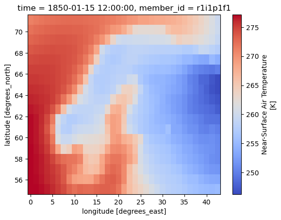
As the exercise is focused on an Area Of Interest, this can be obtained through a bounding box defined with slices.
tas_AOI = tas_ds.tas.sel(lat=slice(54.5,71.5), lon=slice(-2.5,42.5))
tas_AOI
<xarray.DataArray 'tas' (member_id: 1, time: 1980, lat: 18, lon: 35)>
array([[[[277.14154, ..., 255.24866],
         ...,
         [271.17374, ..., 259.73807]],

        ...,

        [[283.0737 , ..., 269.6892 ],
         ...,
         [272.89108, ..., 271.8542 ]]]], dtype=float32)
Coordinates:
  * lat        (lat) float64 55.13 56.07 57.02 57.96 ... 68.32 69.27 70.21 71.15
  * lon        (lon) float64 0.0 1.25 2.5 3.75 5.0 ... 38.75 40.0 41.25 42.5
  * time       (time) object 1850-01-15 12:00:00 ... 2014-12-15 12:00:00
  * member_id  (member_id) object 'r1i1p1f1'
Attributes:
    cell_measures:  area: areacella
    cell_methods:   area: time: mean
    comment:        near-surface (usually, 2 meter) air temperature
    description:    near-surface (usually, 2 meter) air temperature
    frequency:      mon
    id:             tas
    long_name:      Near-Surface Air Temperature
    mipTable:       Amon
    out_name:       tas
    prov:           Amon ((isd.003))
    realm:          atmos
    standard_name:  air_temperature
    time:           time
    time_label:     time-mean
    time_title:     Temporal mean
    title:          Near-Surface Air Temperature
    type:           real
    units:          K
variable_id: tasTip
the values for lat and lon need to be selected in the order shown in the coordinate section (here in increasing order) and not always in increasing order?
You need to use the same order as the corresponding DataArray.
Plotting#
Plotting data can easily be obtained through matplotlib.pyplot back-end matplotlib documentation.
tas_AOI.isel(time=0).plot(cmap="coolwarm")
<matplotlib.collections.QuadMesh at 0x7ff8feff86a0>
In the next episode, we will learn more about advanced visualization tools and how to make interactive plots using holoviews, a tool part of the HoloViz ecosystem.
Basic maths#
Near-surface temperature values are in Kelvin and we can easily convert them in degrees celcius.
Simple arithmetic operations can be performed without worrying about dimensions and coordinates, using the same notation we use with numpy. Underneath xarray will automatically vectorize the operations over all the data dimensions.
tas_AOI - 273.15
<xarray.DataArray 'tas' (member_id: 1, time: 1980, lat: 18, lon: 35)>
array([[[[  3.9915466 ,   3.9372864 ,   3.63208   , ..., -17.947784  ,
          -18.09903   , -17.901337  ],
         [  3.9906616 ,   3.8585205 ,   3.4658813 , ..., -19.287094  ,
          -19.638443  , -19.815659  ],
         [  3.8772888 ,   3.693756  ,   3.3085938 , ..., -20.736603  ,
          -21.195053  , -21.357864  ],
         ...,
         [ -0.11868286,   0.1071167 ,   0.3340149 , ..., -11.844849  ,
          -12.702545  , -14.013733  ],
         [ -0.9946594 ,  -0.6482544 ,  -0.4326172 , ..., -10.813141  ,
          -12.086548  , -13.261871  ],
         [ -1.9762573 ,  -1.6532898 ,  -1.2767944 , ..., -10.560425  ,
          -11.828857  , -13.411926  ]],

        [[  6.5706787 ,   6.261444  ,   5.76593   , ..., -10.512054  ,
          -10.819702  , -11.010132  ],
         [  6.6134033 ,   6.326996  ,   5.8705444 , ..., -10.703583  ,
          -10.812073  , -11.228058  ],
         [  6.63974   ,   6.3713074 ,   5.99823   , ..., -10.811035  ,
          -11.002502  , -11.324585  ],
...
         [  4.5212708 ,   4.881195  ,   5.349457  , ...,  -0.38009644,
           -0.14691162,  -0.15356445],
         [  3.3636475 ,   3.8493652 ,   4.25      , ...,   0.430542  ,
            0.32699585,   0.23458862],
         [  2.291626  ,   2.7035522 ,   3.230133  , ...,   0.6605835 ,
            0.5307617 ,   0.37503052]],

        [[  9.923706  ,  10.213959  ,  10.246948  , ...,  -2.7084656 ,
           -3.117157  ,  -3.460785  ],
         [ 10.048218  ,  10.249817  ,  10.259094  , ...,  -2.855835  ,
           -3.1342468 ,  -3.5550232 ],
         [  9.972595  ,  10.138733  ,  10.1493225 , ...,  -3.176941  ,
           -3.5891113 ,  -3.8943787 ],
         ...,
         [  2.2316895 ,   2.5167236 ,   2.8789368 , ...,  -1.0142822 ,
           -1.0447388 ,  -1.3068542 ],
         [  0.93966675,   1.3753662 ,   1.7021484 , ...,  -0.4562683 ,
           -0.82281494,  -1.1673279 ],
         [ -0.25891113,   0.1281128 ,   0.6257019 , ...,  -0.47140503,
           -0.86395264,  -1.2958069 ]]]], dtype=float32)
Coordinates:
  * lat        (lat) float64 55.13 56.07 57.02 57.96 ... 68.32 69.27 70.21 71.15
  * lon        (lon) float64 0.0 1.25 2.5 3.75 5.0 ... 38.75 40.0 41.25 42.5
  * time       (time) object 1850-01-15 12:00:00 ... 2014-12-15 12:00:00
* member_id (member_id) object 'r1i1p1f1'The universal function (ufunc) from numpy and scipy can be applied too directly to the data. There are currently more than 60 universal functions defined in numpy on one or more types, covering a wide variety of operations including math operations, trigonometric functions, etc.
np.subtract(tas_AOI, 273.15)
<xarray.DataArray 'tas' (member_id: 1, time: 1980, lat: 18, lon: 35)>
array([[[[  3.9915466 ,   3.9372864 ,   3.63208   , ..., -17.947784  ,
          -18.09903   , -17.901337  ],
         [  3.9906616 ,   3.8585205 ,   3.4658813 , ..., -19.287094  ,
          -19.638443  , -19.815659  ],
         [  3.8772888 ,   3.693756  ,   3.3085938 , ..., -20.736603  ,
          -21.195053  , -21.357864  ],
         ...,
         [ -0.11868286,   0.1071167 ,   0.3340149 , ..., -11.844849  ,
          -12.702545  , -14.013733  ],
         [ -0.9946594 ,  -0.6482544 ,  -0.4326172 , ..., -10.813141  ,
          -12.086548  , -13.261871  ],
         [ -1.9762573 ,  -1.6532898 ,  -1.2767944 , ..., -10.560425  ,
          -11.828857  , -13.411926  ]],

        [[  6.5706787 ,   6.261444  ,   5.76593   , ..., -10.512054  ,
          -10.819702  , -11.010132  ],
         [  6.6134033 ,   6.326996  ,   5.8705444 , ..., -10.703583  ,
          -10.812073  , -11.228058  ],
         [  6.63974   ,   6.3713074 ,   5.99823   , ..., -10.811035  ,
          -11.002502  , -11.324585  ],
...
         [  4.5212708 ,   4.881195  ,   5.349457  , ...,  -0.38009644,
           -0.14691162,  -0.15356445],
         [  3.3636475 ,   3.8493652 ,   4.25      , ...,   0.430542  ,
            0.32699585,   0.23458862],
         [  2.291626  ,   2.7035522 ,   3.230133  , ...,   0.6605835 ,
            0.5307617 ,   0.37503052]],

        [[  9.923706  ,  10.213959  ,  10.246948  , ...,  -2.7084656 ,
           -3.117157  ,  -3.460785  ],
         [ 10.048218  ,  10.249817  ,  10.259094  , ...,  -2.855835  ,
           -3.1342468 ,  -3.5550232 ],
         [  9.972595  ,  10.138733  ,  10.1493225 , ...,  -3.176941  ,
           -3.5891113 ,  -3.8943787 ],
         ...,
         [  2.2316895 ,   2.5167236 ,   2.8789368 , ...,  -1.0142822 ,
           -1.0447388 ,  -1.3068542 ],
         [  0.93966675,   1.3753662 ,   1.7021484 , ...,  -0.4562683 ,
           -0.82281494,  -1.1673279 ],
         [ -0.25891113,   0.1281128 ,   0.6257019 , ...,  -0.47140503,
           -0.86395264,  -1.2958069 ]]]], dtype=float32)
Coordinates:
* lat (lat) float64 55.13 56.07 57.02 57.96 ... 68.32 69.27 70.21 71.15
* lon (lon) float64 0.0 1.25 2.5 3.75 5.0 ... 38.75 40.0 41.25 42.5
* time (time) object 1850-01-15 12:00:00 ... 2014-12-15 12:00:00
* member_id (member_id) object 'r1i1p1f1'
Attributes:
cell_measures: area: areacella
cell_methods: area: time: mean
comment: near-surface (usually, 2 meter) air temperature
description: near-surface (usually, 2 meter) air temperature
frequency: mon
id: tas
long_name: Near-Surface Air Temperature
mipTable: Amon
out_name: tas
prov: Amon ((isd.003))
realm: atmos
standard_name: air_temperature
time: time
time_label: time-mean
time_title: Temporal mean
title: Near-Surface Air Temperature
type: real
units: K
variable_id: tastas_AOI = tas_AOI - 273.15
tas_AOI
<xarray.DataArray 'tas' (member_id: 1, time: 1980, lat: 18, lon: 35)>
array([[[[  3.9915466 ,   3.9372864 ,   3.63208   , ..., -17.947784  ,
          -18.09903   , -17.901337  ],
         [  3.9906616 ,   3.8585205 ,   3.4658813 , ..., -19.287094  ,
          -19.638443  , -19.815659  ],
         [  3.8772888 ,   3.693756  ,   3.3085938 , ..., -20.736603  ,
          -21.195053  , -21.357864  ],
         ...,
         [ -0.11868286,   0.1071167 ,   0.3340149 , ..., -11.844849  ,
          -12.702545  , -14.013733  ],
         [ -0.9946594 ,  -0.6482544 ,  -0.4326172 , ..., -10.813141  ,
          -12.086548  , -13.261871  ],
         [ -1.9762573 ,  -1.6532898 ,  -1.2767944 , ..., -10.560425  ,
          -11.828857  , -13.411926  ]],

        [[  6.5706787 ,   6.261444  ,   5.76593   , ..., -10.512054  ,
          -10.819702  , -11.010132  ],
         [  6.6134033 ,   6.326996  ,   5.8705444 , ..., -10.703583  ,
          -10.812073  , -11.228058  ],
         [  6.63974   ,   6.3713074 ,   5.99823   , ..., -10.811035  ,
          -11.002502  , -11.324585  ],
...
         [  4.5212708 ,   4.881195  ,   5.349457  , ...,  -0.38009644,
           -0.14691162,  -0.15356445],
         [  3.3636475 ,   3.8493652 ,   4.25      , ...,   0.430542  ,
            0.32699585,   0.23458862],
         [  2.291626  ,   2.7035522 ,   3.230133  , ...,   0.6605835 ,
            0.5307617 ,   0.37503052]],

        [[  9.923706  ,  10.213959  ,  10.246948  , ...,  -2.7084656 ,
           -3.117157  ,  -3.460785  ],
         [ 10.048218  ,  10.249817  ,  10.259094  , ...,  -2.855835  ,
           -3.1342468 ,  -3.5550232 ],
         [  9.972595  ,  10.138733  ,  10.1493225 , ...,  -3.176941  ,
           -3.5891113 ,  -3.8943787 ],
         ...,
         [  2.2316895 ,   2.5167236 ,   2.8789368 , ...,  -1.0142822 ,
           -1.0447388 ,  -1.3068542 ],
         [  0.93966675,   1.3753662 ,   1.7021484 , ...,  -0.4562683 ,
           -0.82281494,  -1.1673279 ],
         [ -0.25891113,   0.1281128 ,   0.6257019 , ...,  -0.47140503,
           -0.86395264,  -1.2958069 ]]]], dtype=float32)
Coordinates:
* lat (lat) float64 55.13 56.07 57.02 57.96 ... 68.32 69.27 70.21 71.15
* lon (lon) float64 0.0 1.25 2.5 3.75 5.0 ... 38.75 40.0 41.25 42.5
* time (time) object 1850-01-15 12:00:00 ... 2014-12-15 12:00:00
* member_id (member_id) object 'r1i1p1f1'Statistics#
All the standard statistical operations can be used such as min, max, mean. When no argument is passed to the function, the operation is done over all the dimensions of the variable (same as with numpy).
tas_AOI.min()
<xarray.DataArray 'tas' ()>
array(-26.84191895)
You can make a statistical operation over a dimension. For instance, let’s retrieve the maximum tas value among all those available for different times, at each lat-lon location.
tas_AOI.max(dim='time')
<xarray.DataArray 'tas' (member_id: 1, lat: 18, lon: 35)>
array([[[17.913177 , 18.16388  , 18.275024 , 18.313934 , 18.328522 ,
         18.410065 , 18.476685 , 19.338104 , 20.345673 , 19.73639  ,
         19.681091 , 20.134735 , 19.119598 , 19.005066 , 19.041931 ,
         19.106995 , 19.019653 , 22.693756 , 24.226562 , 24.650146 ,
         24.417786 , 23.973938 , 23.803497 , 22.828125 , 22.704803 ,
         22.352753 , 22.175903 , 22.134857 , 23.450043 , 24.378357 ,
         25.166748 , 25.610962 , 24.972687 , 25.00238  , 24.528198 ],
        [17.241577 , 17.338257 , 17.492157 , 17.585663 , 17.65509  ,
         17.713348 , 17.98352  , 20.150513 , 21.748383 , 21.886383 ,
         21.556824 , 20.893677 , 20.363037 , 18.943329 , 18.613983 ,
         18.611572 , 18.620941 , 19.760834 , 23.221924 , 23.647827 ,
         23.514404 , 23.093231 , 23.336456 , 22.503937 , 22.339935 ,
         22.338959 , 22.166626 , 22.34134  , 23.142212 , 23.4458   ,
         24.20691  , 24.140076 , 24.62323  , 24.352112 , 24.227814 ],
        [16.807587 , 16.770233 , 16.859833 , 16.93045  , 16.981567 ,
         17.039246 , 17.455383 , 18.455078 , 19.253387 , 20.740967 ,
         21.366882 , 21.06958  , 20.757294 , 20.318634 , 18.286224 ,
         18.358154 , 18.349121 , 19.311615 , 21.430908 , 22.219482 ,
         22.33014  , 22.559174 , 22.694366 , 22.51947  , 22.080627 ,
         22.51355  , 22.614471 , 22.480713 , 22.66214  , 23.090118 ,
...
         12.900909 , 13.222961 , 13.52597  , 14.403259 , 15.553009 ,
         16.8042   , 16.932892 , 16.954376 , 17.034729 , 16.96762  ,
         16.96637  , 17.100616 , 17.330872 , 17.345306 , 17.114044 ,
         16.488129 , 14.975281 , 12.001068 , 13.143677 , 10.707916 ,
          9.694275 ,  9.177216 ,  9.027313 ,  8.803345 ,  8.669434 ],
        [ 9.139069 ,  9.590576 ,  9.904144 , 10.247589 , 10.48056  ,
         10.866425 , 11.181763 , 11.512421 , 11.786804 , 12.199493 ,
         12.608215 , 12.951721 , 13.20874  , 13.357086 , 13.322723 ,
         14.709045 , 13.948395 , 15.049042 , 16.412964 , 17.884033 ,
         17.783173 , 17.81784  , 17.365814 , 17.036255 , 16.102875 ,
         12.359375 ,  9.921783 ,  9.611908 ,  9.409424 ,  9.122467 ,
          8.811737 ,  8.50293  ,  8.18045  ,  7.9012146,  7.5783386],
        [ 8.040253 ,  8.353821 ,  8.763489 ,  9.011475 ,  9.314575 ,
          9.718872 , 10.178741 , 10.651154 , 11.184814 , 11.681763 ,
         12.085083 , 12.411102 , 12.637634 , 12.749329 , 12.723297 ,
         12.770172 , 12.895966 , 12.92099  , 12.873657 , 13.131958 ,
         14.395782 , 12.900848 , 12.762329 , 11.248535 , 10.335876 ,
          9.764557 ,  9.28595  ,  8.989227 ,  8.640686 ,  8.288513 ,
          7.905426 ,  7.5679626,  7.2664795,  7.0660706,  6.9654236]]],
      dtype=float32)
Coordinates:
  * lat        (lat) float64 55.13 56.07 57.02 57.96 ... 68.32 69.27 70.21 71.15
  * lon        (lon) float64 0.0 1.25 2.5 3.75 5.0 ... 38.75 40.0 41.25 42.5
* member_id (member_id) object 'r1i1p1f1'Aggregation#
We have monthly data. To obtain yearly values, we can group values per year and compute the mean.
tas_yearly = tas_AOI.groupby(tas_AOI.time.dt.year).mean()
tas_yearly
<xarray.DataArray 'tas' (member_id: 1, year: 165, lat: 18, lon: 35)>
array([[[[10.190738  , 10.236267  , 10.129463  , ...,  4.487551  ,
           4.577349  ,  4.4684777 ],
         [10.055203  , 10.016124  ,  9.869583  , ...,  3.5996563 ,
           3.602525  ,  3.5518277 ],
         [ 9.951228  ,  9.84331   ,  9.695267  , ...,  2.8245113 ,
           2.760255  ,  2.7445972 ],
         ...,
         [ 2.131218  ,  2.480194  ,  2.8605297 , ..., -4.5990014 ,
          -4.9325995 , -5.297928  ],
         [ 0.8806508 ,  1.3956375 ,  1.7613932 , ..., -4.671717  ,
          -5.130834  , -5.525271  ],
         [-0.27815247,  0.1952184 ,  0.7522685 , ..., -4.968567  ,
          -5.4446716 , -5.893354  ]],

        [[10.707288  , 10.862836  , 10.859578  , ...,  7.673986  ,
           7.586838  ,  7.378306  ],
         [10.575684  , 10.646342  , 10.60096   , ...,  7.274389  ,
           7.101011  ,  6.786873  ],
         [10.451709  , 10.4361925 , 10.362701  , ...,  6.5675125 ,
           6.483808  ,  6.3353195 ],
...
         [ 3.899109  ,  4.278895  ,  4.683767  , ...,  0.22347514,
           0.07540639, -0.13505554],
         [ 2.6409404 ,  3.1836903 ,  3.5581539 , ...,  0.25100455,
          -0.05962372, -0.3530426 ],
         [ 1.38296   ,  1.857727  ,  2.4163895 , ...,  0.07100169,
          -0.25650534, -0.61615247]],

        [[11.859332  , 12.051389  , 12.075607  , ...,  8.140752  ,
           8.121837  ,  7.935308  ],
         [11.677655  , 11.791171  , 11.787402  , ...,  7.7124076 ,
           7.5722404 ,  7.4204307 ],
         [11.52195   , 11.550827  , 11.534116  , ...,  7.284935  ,
           7.149447  ,  7.030052  ],
         ...,
         [ 4.1399918 ,  4.518181  ,  4.9494348 , ...,  1.4126383 ,
           1.2889252 ,  1.1015829 ],
         [ 2.8445637 ,  3.3857346 ,  3.787501  , ...,  1.4600092 ,
           1.1696981 ,  0.8996175 ],
         [ 1.5644354 ,  2.0351918 ,  2.6172917 , ...,  1.269165  ,
           0.9806595 ,  0.6546936 ]]]], dtype=float32)
Coordinates:
  * lat        (lat) float64 55.13 56.07 57.02 57.96 ... 68.32 69.27 70.21 71.15
  * lon        (lon) float64 0.0 1.25 2.5 3.75 5.0 ... 38.75 40.0 41.25 42.5
  * member_id  (member_id) object 'r1i1p1f1'
* year (year) int64 1850 1851 1852 1853 1854 ... 2011 2012 2013 2014As we have data from 1850 to 2014, the time dimension is now year and takes values from 1850 to 2014.
tas_yearly.year
<xarray.DataArray 'year' (year: 165)>
array([1850, 1851, 1852, 1853, 1854, 1855, 1856, 1857, 1858, 1859, 1860, 1861,
       1862, 1863, 1864, 1865, 1866, 1867, 1868, 1869, 1870, 1871, 1872, 1873,
       1874, 1875, 1876, 1877, 1878, 1879, 1880, 1881, 1882, 1883, 1884, 1885,
       1886, 1887, 1888, 1889, 1890, 1891, 1892, 1893, 1894, 1895, 1896, 1897,
       1898, 1899, 1900, 1901, 1902, 1903, 1904, 1905, 1906, 1907, 1908, 1909,
       1910, 1911, 1912, 1913, 1914, 1915, 1916, 1917, 1918, 1919, 1920, 1921,
       1922, 1923, 1924, 1925, 1926, 1927, 1928, 1929, 1930, 1931, 1932, 1933,
       1934, 1935, 1936, 1937, 1938, 1939, 1940, 1941, 1942, 1943, 1944, 1945,
       1946, 1947, 1948, 1949, 1950, 1951, 1952, 1953, 1954, 1955, 1956, 1957,
       1958, 1959, 1960, 1961, 1962, 1963, 1964, 1965, 1966, 1967, 1968, 1969,
       1970, 1971, 1972, 1973, 1974, 1975, 1976, 1977, 1978, 1979, 1980, 1981,
       1982, 1983, 1984, 1985, 1986, 1987, 1988, 1989, 1990, 1991, 1992, 1993,
       1994, 1995, 1996, 1997, 1998, 1999, 2000, 2001, 2002, 2003, 2004, 2005,
       2006, 2007, 2008, 2009, 2010, 2011, 2012, 2013, 2014])
Coordinates:
* year (year) int64 1850 1851 1852 1853 1854 ... 2010 2011 2012 2013 2014Mask#
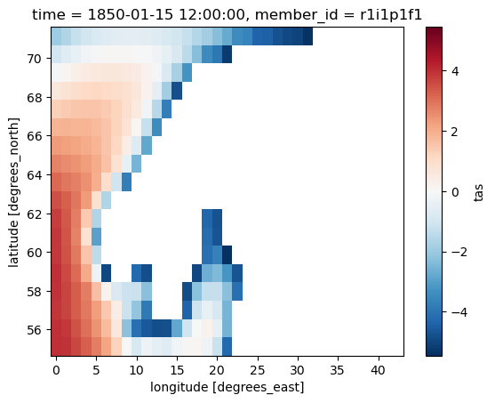
Masking can be achieved through the method DataSet|Array.where(cond, other) or xr.where(cond, x, y).
The difference consists in the possibility to specify the value in case the condition is positive or not; DataSet|Array.where(cond, other) only offer the possibility to define the false condition value (by default is set to np.NaN))
tas_masked = tas_AOI.where((tas_AOI >= -5.5) & (tas_AOI <= 15))
tas_masked.isel(time=0).plot()
<matplotlib.collections.QuadMesh at 0x7ff8f5fc4df0>
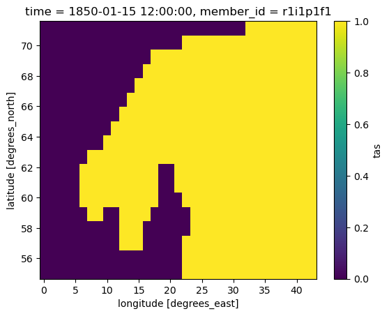
To better visualize the mask, with the help of xr.where, ad-hoc variables can be created. ‘xr.where’ lets us specify values of 1 for masked and 0 for the unmasked data.
mask = xr.where((tas_AOI <= -5.5) | (tas_AOI >= 15), 1, 0)
mask.isel(time=0).plot()
<matplotlib.collections.QuadMesh at 0x7ff8f5eca880>
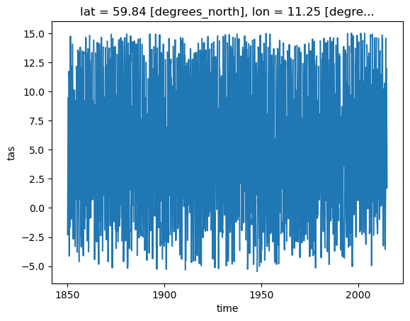
Plot a single point (defined by its latitude and longitude) over the time dimension.
tas_masked.sel(lat=60., lon=10.75, method='nearest').plot()
[<matplotlib.lines.Line2D at 0x7ff8f5e6bb50>]
Save xarray Dataset#
It is very often convenient to save intermediate or final results into a local file. We will learn more about the different file formats Xarray can handle, but for now let’s save it as a netCDF file. Check the file size after saving the result into netCDF.
tas_masked.to_netcdf('tas_Nordic_masked.nc')
Advanced Saving methods#
Encoding and Compression#
From the near-surface temperature dataset we already know that values are encoded as float32. A compression method can be defined as well; if the format is netCDF4 with the engine set to ‘netcdf4’ or ‘h5netcdf’ there are different compression options. The easiest solution is to stick with the default one for NetCDF4 files.
Note that encoding parameters needs to be done through a nested dictionary and parameters has to be defined for each single variable.
tas_masked.to_netcdf('tas_Nordic_mcs.nc',
                      engine='netcdf4',
                      encoding={'tas':{"dtype": np.float32,
                                        'zlib': True, 'complevel':4}
                                }
                      )
- Xarray Dataset and DataArray
- Read and get metadata from local raster file
- Dataset and DataArray selection
- Aggregation and statistics
- Masking values
Through the datatype and the compression a compression of almost 10 time has been achieved; as drawback speed reading has been decreased.
References#
- Kog95
F.N. Kogan. Application of vegetation index and brightness temperature for drought detection. Advances in Space Research, 15(11):91–100, 1995. Natural Hazards: Monitoring and Assessment Using Remote Sensing Technique. URL: https://www.sciencedirect.com/science/article/pii/027311779500079T, doi:https://doi.org/10.1016/0273-1177(95)00079-T.
- Wik2)
Wikipedia. Normalized difference vegetation index. https://en.wikipedia.org/wiki/Normalized_difference_vegetation_index, 2022 (accessed August 7, 2022).
Packages citation#
- HMvdW+20
Charles R. Harris, K. Jarrod Millman, Stéfan J. van der Walt, Ralf Gommers, Pauli Virtanen, David Cournapeau, Eric Wieser, Julian Taylor, Sebastian Berg, Nathaniel J. Smith, Robert Kern, Matti Picus, Stephan Hoyer, Marten H. van Kerkwijk, Matthew Brett, Allan Haldane, Jaime Fernández del Río, Mark Wiebe, Pearu Peterson, Pierre Gérard-Marchant, Kevin Sheppard, Tyler Reddy, Warren Weckesser, Hameer Abbasi, Christoph Gohlke, and Travis E. Oliphant. Array programming with NumPy. Nature, 585(7825):357–362, September 2020. URL: https://doi.org/10.1038/s41586-020-2649-2, doi:10.1038/s41586-020-2649-2.
- HH17
S. Hoyer and J. Hamman. Xarray: N-D labeled arrays and datasets in Python. Journal of Open Research Software, 2017. URL: https://doi.org/10.5334/jors.148, doi:10.5334/jors.148.
- USR+20
Leonardo Uieda, Santiago Rubén Soler, Rémi Rampin, Hugo van Kemenade, Matthew Turk, Daniel Shapero, Anderson Banihirwe, and John Leeman. Pooch: a friend to fetch your data files. Journal of Open Source Software, 5(45):1943, 2020. URL: https://doi.org/10.21105/joss.01943, doi:10.21105/joss.01943.