Interactive plotting with HoloViews#
Context#
We will be using HoloViews, a tool part of the HoloViz ecosystem, with Xarray to visualize the Vegetation Condition Index (VCI) [Kog95], a well-established indicator to estimate droughts from remote sensing data.
Data#
We will use data that have been generated in the previous episode.
If the dataset is not present in the same folder as this Jupyter notebook, it will be downloaded from zenodo using pooch, a very handy python-based library to download and cache your data files locally (see further info here).
import pooch
cgls_file = pooch.retrieve(
url="https://zenodo.org/record/6969999/files/C_GLS_NDVI_20220101_20220701_Lombardia_S3_2_masked.nc",
known_hash="md5:be3f16913ebbdb4e7af227f971007b22",
path=f".",
)
Downloading data from 'https://zenodo.org/record/6969999/files/C_GLS_NDVI_20220101_20220701_Lombardia_S3_2_masked.nc' to file '/home/runner/work/pangeo-openeo-BiDS-2023/pangeo-openeo-BiDS-2023/tutorial/part1/3bcb6b0879f7f1f3eebff65b142241cf-C_GLS_NDVI_20220101_20220701_Lombardia_S3_2_masked.nc'.
Setup#
This episode uses the following main Python packages:
pooch [USR+20]
rioxarray [SBR+22]
matplotlib [Hun07]
cartopy [MetOffice15]
hvplot [RSB+20]
geopandas [JdBF+20]
Please install these packages if not already available in your Python environment.
Packages#
In this episode, Python packages are imported when we start to use them. However, for best software practices, we recommend you to install and import all the necessary libraries at the top of your Jupyter notebook.
import xarray as xr
Open local dataset#
cgls_ds = xr.open_dataset(cgls_file)
Tip
If you get an error with the previous command, check the previous episode where the input file some_hash-C_GLS_NDVI_20220101_20220701_Lombardia_S3_2_masked.netcdf is downloaded locally and it is in the same directory as your Jupyter Notebook.
cgls_ds
<xarray.Dataset> Size: 96MB
Dimensions: (time: 20, lon: 984, lat: 612)
Coordinates:
* time (time) datetime64[ns] 160B 2022-01-01 2022-01-11 ... 2022-07-11
* lon (lon) float64 8kB 8.502 8.505 8.508 8.511 ... 11.42 11.42 11.43
* lat (lat) float64 5kB 46.5 46.5 46.49 46.49 ... 44.69 44.69 44.68 44.68
Data variables:
NDVI (time, lat, lon) float64 96MB ...Clipping data according to a polygon#
One of the basic concepts in GIS is to clip data using a vector geometry. Xarray is not directly capable of dealing with vectors but thanks to Rioxarray that can be easily achieved. Rioxarray extends Xarray with most of the features that Rasterio (GDAL) brings.
Read a shapefile with the Area Of Interest (AOI)#
import geopandas as gpd
We define the area of interest using the Global Administrative Unit Layers GAUL G2015_2014 provided by FAO-UN (see Documentation).
GeoPandas, a python-based library extending the capabilities of Pandas to deal with geometry and spatial operations, will help to manage geodata.
The official data distribution from FAO is through the WFS service (see below how to retrieve data):
GAUL = gpd.read_file('https://data.apps.fao.org/map/gsrv/gsrv1/gaul/wfs?'
'service=WFS&version=2.0.0&'
'Request=GetFeature&'
'TypeNames=gaul:g2015_2014_2&'
'srsName=EPSG%3A4326&'
'maxFeatures=2500&'
'outputFormat=json')
Unfortunately it seems that the service is pretty slow. As an alternative to this approach the JRC MARS unit is distributing the original dataset that was in shapefile format. To accelerate the fetch we highly recommend to follow this approach.
For the training course, we also created a tiny file containing information about Italy only.
try:
GAUL = gpd.read_file('Italy.geojson')
except:
GAUL = gpd.read_file('zip+https://agricultural-production-hotspots.ec.europa.eu/files/gaul1_asap.zip')
Data are organized in a tabular structure. For each element an index, data (made of columns) and a geometry are defined.
Geometries are defined through shapely geometry objects with three different basic classes:
Points and Multi-Points
Lines and Multi-Lines
Polygons and Multi-Polygons
GAUL.head(5)
| asap1_id | name1 | name1_shr | name0 | asap0_id | name0_shr | km2_tot | km2_crop | km2_range | an_crop | an_range | water_lim | geometry | |
|---|---|---|---|---|---|---|---|---|---|---|---|---|---|
| 0 | 263 | Damietta | Damietta | Egypt | 79 | Egypt | 928 | 550 | 0 | 1 | 0 | 1 | POLYGON ((31.84469 31.52698, 31.84601 31.52356... |
| 1 | 2141 | Ninh Binh | Ninh Binh | Viet Nam | 134 | Viet Nam | 1362 | 1035 | 80 | 1 | 0 | 0 | POLYGON ((105.77766 20.43617, 105.77976 20.435... |
| 2 | 10070 | Segen Peoples | Segen Peoples | Ethiopia | 185 | Ethiopia | 6813 | 382 | 6288 | 1 | 1 | 1 | POLYGON ((37.90356 5.95984, 37.92241 5.95941, ... |
| 3 | 2150 | Thai Binh | Thai Binh | Viet Nam | 134 | Viet Nam | 1559 | 1189 | 51 | 1 | 0 | 0 | POLYGON ((106.41657 20.71235, 106.41279 20.711... |
| 4 | 2001 | Tekirdag | Tekirdag | Turkey | 49 | Turkey | 6237 | 4561 | 1188 | 1 | 1 | 1 | POLYGON ((28.16894 41.47137, 28.18175 41.46005... |
In the cell below, we subset the polygon geometry in which the name1 field equals to Lombardia.
AOI_name = 'Lombardia'
AOI = GAUL[GAUL.name1 == AOI_name]
AOI_poly = AOI.geometry
AOI_poly
1755 POLYGON ((10.23973 46.62177, 10.25084 46.61110...
Name: geometry, dtype: geometry
In a second step we set a EPSG:4326 Geodetic coordinate reference system to the polygon geometry. To achieve this we need to rely on rioxarray that extends xarray with the rasterio capabilities. The rio accessor is activated through importing rioxarray as has been done at the top.
cgls_ds.rio.write_crs(4326, inplace=True)
<xarray.Dataset> Size: 96MB
Dimensions: (time: 20, lon: 984, lat: 612)
Coordinates:
* time (time) datetime64[ns] 160B 2022-01-01 2022-01-11 ... 2022-07-11
* lon (lon) float64 8kB 8.502 8.505 8.508 8.511 ... 11.42 11.42 11.43
* lat (lat) float64 5kB 46.5 46.5 46.49 46.49 ... 44.69 44.68 44.68
spatial_ref int64 8B 0
Data variables:
NDVI (time, lat, lon) float64 96MB ...Once this has been done we can clip the data with the polygon that has been obtained through geopandas at the beginning of the notebook.
NDVI_AOI = cgls_ds.NDVI.rio.clip(AOI_poly, crs=4326)
Visualize with matplotlib#
import matplotlib.pyplot as plt
import cartopy.crs as ccrs
fig = plt.figure(1, figsize=[20, 10])
# We're using cartopy and are plotting in PlateCarree projection
# (see documentation on cartopy)
ax = plt.subplot(1, 1, 1, projection=ccrs.PlateCarree())
#ax.set_extent([15.5, 27.5, 36, 41], crs=ccrs.PlateCarree()) # lon1 lon2 lat1 lat2
ax.coastlines(resolution='10m')
ax.gridlines(draw_labels=True)
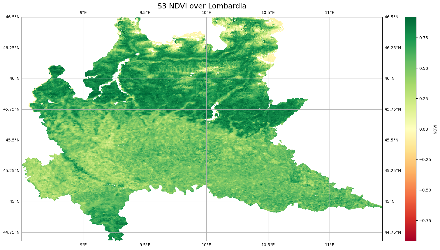
NDVI_AOI.sel(time='2022-06-01').plot(ax=ax, transform=ccrs.PlateCarree(), cmap="RdYlGn")
# One way to customize your title
plt.title("S3 NDVI over Lombardia", fontsize=18)
Text(0.5, 1.0, 'S3 NDVI over Lombardia')
/home/runner/micromamba/envs/bids23/lib/python3.11/site-packages/cartopy/io/__init__.py:241: DownloadWarning: Downloading: https://naturalearth.s3.amazonaws.com/10m_physical/ne_10m_coastline.zip
warnings.warn(f'Downloading: {url}', DownloadWarning)
Visualization with HoloViews#
import holoviews as hv
import hvplot.xarray
import hvplot.pandas
Plotting data through the HoloViews back-end thanks to the hvplot that acts as high-level plotting API.
NDVI_AOI.isel(time=0).hvplot(cmap="RdYlGn", width=1000, height=1000)
Having a look to data distribution can reveal a lot about the data.
NDVI_AOI[0].hvplot.hist(cmap="RdYlGn",bins=25, width=800, height=700)
Multi-plots using groupby#
To be able to visualize interactively all the different available times, we can use groupby time.
NDVI_AOI.hvplot(groupby ='time', cmap="RdYlGn", width=800, height=700)
We can add a histogram to the visualization.
NDVI_AOI.hvplot(groupby='time', cmap='RdYlGn', width=800, height=700 ).hist()
Plot a single point over the time dimension#
NDVI_AOI.sel(lat=45.88, lon=8.63, method='nearest').hvplot(ylim=(-0.08, 0.92))
- Rioxarray for clipping over an area of interest
- Interactive plot with HoloViews and Xarray
References#
F.N. Kogan. Application of vegetation index and brightness temperature for drought detection. Advances in Space Research, 15(11):91–100, 1995. Natural Hazards: Monitoring and Assessment Using Remote Sensing Technique. URL: https://www.sciencedirect.com/science/article/pii/027311779500079T, doi:https://doi.org/10.1016/0273-1177(95)00079-T.
Packages citation#
S. Hoyer and J. Hamman. Xarray: N-D labeled arrays and datasets in Python. Journal of Open Research Software, 2017. URL: https://doi.org/10.5334/jors.148, doi:10.5334/jors.148.
J. D. Hunter. Matplotlib: a 2d graphics environment. Computing in Science & Engineering, 9(3):90–95, 2007. doi:10.1109/MCSE.2007.55.
Kelsey Jordahl, Joris Van den Bossche, Martin Fleischmann, Jacob Wasserman, James McBride, Jeffrey Gerard, Jeff Tratner, Matthew Perry, Adrian Garcia Badaracco, Carson Farmer, Geir Arne Hjelle, Alan D. Snow, Micah Cochran, Sean Gillies, Lucas Culbertson, Matt Bartos, Nick Eubank, maxalbert, Aleksey Bilogur, Sergio Rey, Christopher Ren, Dani Arribas-Bel, Leah Wasser, Levi John Wolf, Martin Journois, Joshua Wilson, Adam Greenhall, Chris Holdgraf, Filipe, and François Leblanc. Geopandas/geopandas: v0.8.1. July 2020. URL: https://doi.org/10.5281/zenodo.3946761, doi:10.5281/zenodo.3946761.
Philipp Rudiger, Jean-Luc Stevens, James A. Bednar, Bas Nijholt, Andrew, Chris B, Achim Randelhoff, Jon Mease, Vasco Tenner, maxalbert, Markus Kaiser, ea42gh, Jordan Samuels, stonebig, Florian LB, Andrew Tolmie, Daniel Stephan, Scott Lowe, John Bampton, henriqueribeiro, Irv Lustig, Julia Signell, Justin Bois, Leopold Talirz, Lukas Barth, Maxime Liquet, Ram Rachum, Yuval Langer, arabidopsis, and kbowen. Holoviz/holoviews: version 1.13.3. June 2020. URL: https://doi.org/10.5281/zenodo.3904606, doi:10.5281/zenodo.3904606.
Alan D. Snow, David Brochart, Martin Raspaud, Ray Bell, RichardScottOZ, Taher Chegini, Alessandro Amici, Rémi Braun, Andrew Annex, David Hoese, Fred Bunt, GBallesteros, Joe Hamman, Markus Zehner, Mauricio Cordeiro, Scott Henderson, Seth Miller, The Gitter Badger, Tom Augspurger, apiwat-chantawibul, and pmallas. Corteva/rioxarray: 0.11.1 release. April 2022. URL: https://doi.org/10.5281/zenodo.6478182, doi:10.5281/zenodo.6478182.
Leonardo Uieda, Santiago Rubén Soler, Rémi Rampin, Hugo van Kemenade, Matthew Turk, Daniel Shapero, Anderson Banihirwe, and John Leeman. Pooch: a friend to fetch your data files. Journal of Open Source Software, 5(45):1943, 2020. URL: https://doi.org/10.21105/joss.01943, doi:10.21105/joss.01943.
Met Office. Cartopy: a cartographic python library with a matplotlib interface. Exeter, Devon, 2010 - 2015. URL: http://scitools.org.uk/cartopy.