
Scaling openEO & under the hood#
To understand how the design of openEO is linked to performance and scalability, this page is a good read.
Under the hood#
openEO backends rely on the same principles as e.g. Dask and any other large scale parallel processing framework:
The ‘map/reduce’ paradigm
Data ‘partitioning’
As openEO user, you don’t really need to fully understand these things, but it can be useful to better understand performance. We give some examples:
An ‘apply’ process like 2*band_value is very efficient because each pixel can be processed independently. A process like ‘apply_dimension’ over time can require the data to be reshuffled so it can be quite cost intensive over long time series. Aggregate_spatial with a sum over pixels can be implemented as a ‘reduce’ style operation, making it again relatively efficient.
Data partitioning is also something that a backend normally does for you, but it may happen that it is not ‘smart enough’ to understand your use case.This can lead for instance to ‘out of memory’ style errors.
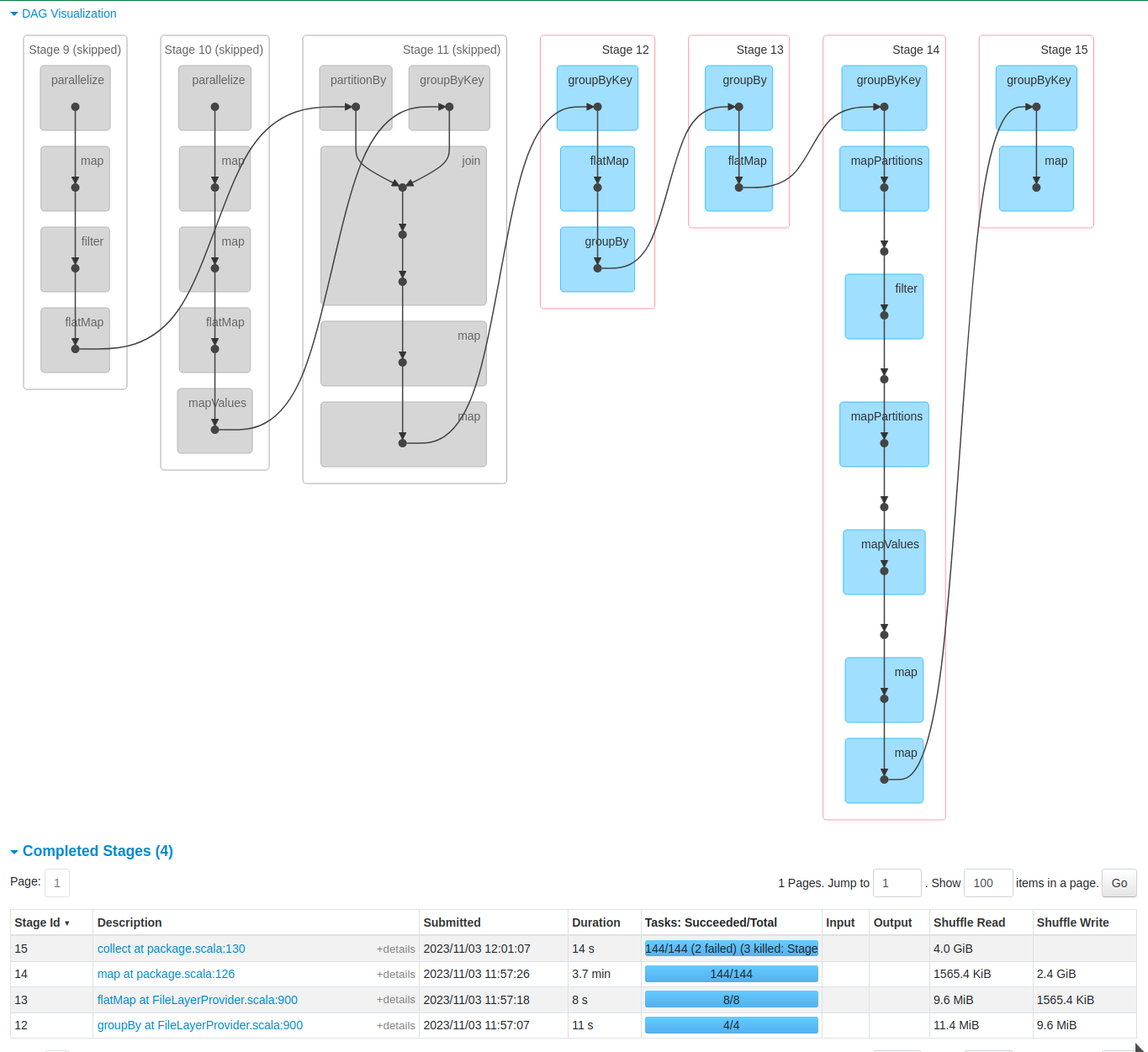
In a real world backend, these concepts result in a graph of processing steps (‘stages’ in Spark), and a number of tasks per step that can be executed in parallel. An example is shown below.
Performance: why does it take so long for openEO to retrieve a simple timeseries?#
What you may notice when working with an openEO backend, is that it can take up to a few minutes to retrieve a ‘simple’ timeseries of for instance Sentinel-2 data. While when loading that timeseries from a netCDF file on your laptop, it’s instantaneous. For many, this is annoying when trying to work interactively, and openEO advices to use the ‘local processing’ feature. So what is going on here?
Warning: this answer is about a specific, but fairly common, backend setup. It does not reflect a general limitation in the openEO design!
The problem is that large EO archives, like Copernicus Sentinel-2 and Sentinel-1, but also Landsat, are stored per ‘product’ on large scale storage systems that are accessed over a network. The consequence is that in most EO-workflows, loading the data (IO) remains the big bottleneck. So while many algorithm writers focus on the processing performance, it is often reading data from 1000’s of files (e.g. 10 bands x 100 observations) over a network that takes most time.
When your multiband timeseries is stored as a single netCDF file on the SSD of your laptop, most of the heavy lifting has in fact been done, because you then have something that can be read into memory at once in a second or less.
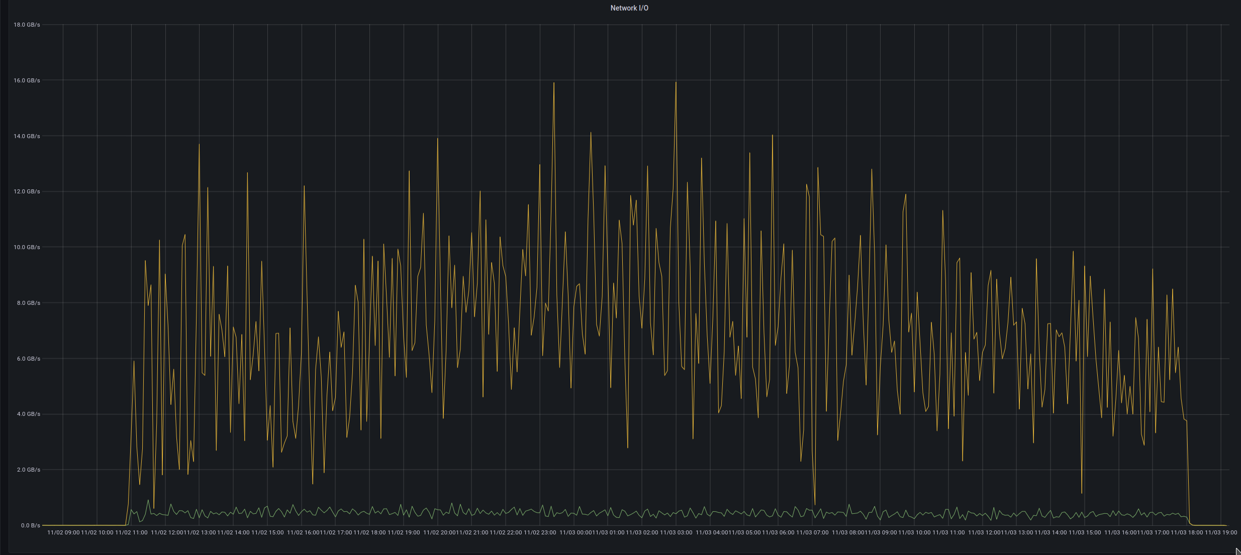
So does this mean that you are better off downloading everything locally and processing on your own resources? In fact not, the graph below shows the reading speed of an openEO cluster that is processing a number of batch jobs. As you can see, in this case it was able to read from EO data at speeds between 4 GB/s and 10 GB/s, which will be hard to achieve when going over the internet.
Example architecture#
There is no single openEO architecture, as openEO is just an API that can be implemented on top of many technologies. That is also a key point which makes it technology independent.
The image shown below shows a typical ‘cloud’ deployment in a Kubernetes environment. Cloud based environments tend to use automatic scaling techniques to grow or shrink the size of the openEO backend based on the requests from users.

Understanding logs#
An openEO backend provides logging, but it can be particularly hard to understand. This again has to do with the cloud based nature: when running your job on many machines in parallel, all kinds of ‘warnings’ and even ‘error’ messages can be generated. There is however a level of fault-tolerance, so there may be errors that are not actually an issue, or there may be errors caused later on, where the actual cause was logged earlier.
So in general, it can help to look for those earliest errors if you see a lot of confusing messages. The log level filtering functionality can help you to do that.
General performance tips#
Keep the size of your data cube in mind#
Backends are distributed, cloud based programs, but it is still possible to overload them easily due to the sheer size of earth observation datasets. If your algorithm at some point reduces dataset size, you may want to put this step early in the algorithm.
Some typical examples:
cloud filtering
masking on a specific landcover type. (e.g. filtering on forest pixels only when you work on a forest app)
reducing temporal resolution, e.g. 10-daily or monthly compositing
reducing resolution
fiter on bands, orbit direction, …
Try to keep the graph simple#
Backends may try to ‘understand’ your process graph, to choose the most optimal evaluation path. Sometimes people introduce an unneeded amount of ‘merge_cubes’ processes, and the graph starts to look quite complex. At this point, also the backend may have trouble understanding this, and your execution is also slow.
Data collection types#
While openEO offers access to many different collections, not all of them use optimal formats or are stored close to the processing center. The result is that there can be quite large difference in performance depending on which collection you use. Hence, it may be smart to check with your backend provider on the specifics of a given collection before trying to use it at scale.
Continental scale processing#
Reference: https://docs.openeo.cloud/usecases/large-scale-processing/