openEO Platform

Big Data From Space 2023

Exploring bottom of atmosphere data

Connect to openEO Platform using python

import openeo
from openeo.processes import *

conn = openeo.connect("openeo.cloud") 

conn = conn.authenticate_oidc()

Authenticated using refresh token.

Look at the collection description

conn.describe_collection("boa_sentinel_2")

Start creating an openEO process graph

Pick a spatial extent of interest

spatial_extent = {'west': 16.2401, 'south': 48.1541, 'east': 16.5595, 'north': 48.2458}

Load the bottom of atmosphere Sentinel 2 collection

data = conn.load_collection('boa_sentinel_2', spatial_extent = spatial_extent, temporal_extent = ["2020-02-01","2020-12-01"], bands=["B02","B03","B04"])

Aggregate the data for one month using a median

data_t = data.aggregate_temporal_period(period="month", reducer=median)

Save the result as a netCDF

saved_data = data_t.save_result(format="NetCDF")
saved_data.flat_graph()

{'loadcollection1': {'process_id': 'load_collection',
  'arguments': {'bands': ['B02', 'B03', 'B04'],
   'id': 'boa_sentinel_2',
   'spatial_extent': {'west': 16.2401,
    'south': 48.1541,
    'east': 16.5595,
    'north': 48.2458},
   'temporal_extent': ['2020-02-01', '2020-12-01']}},
 'aggregatetemporalperiod1': {'process_id': 'aggregate_temporal_period',
  'arguments': {'data': {'from_node': 'loadcollection1'},
   'period': 'month',
   'reducer': {'process_graph': {'median1': {'process_id': 'median',
      'arguments': {'data': {'from_parameter': 'data'}},
      'result': True}}}}},
 'saveresult1': {'process_id': 'save_result',
  'arguments': {'data': {'from_node': 'aggregatetemporalperiod1'},
   'format': 'NetCDF',
   'options': {}},
  'result': True}}

Create and start a job

job = saved_data.create_job()
job.start_job()

job

Download the results, when the job is finished

Look at the results using python matplotlib

from utils import *

path = "./boa/"
output_s2 = load_data(path)

output_s2

<xarray.Dataset>
Dimensions:      (t: 10, y: 1262, x: 2468)
Coordinates:
  * y            (y) float64 1.623e+06 1.623e+06 1.623e+06 ... 1.61e+06 1.61e+06
  * x            (x) float64 5.26e+06 5.26e+06 5.26e+06 ... 5.285e+06 5.285e+06
    spatial_ref  int32 0
  * t            (t) datetime64[ns] 2020-02-29 2020-03-31 ... 2020-11-30
Data variables:
    B02          (t, y, x) float32 dask.array<chunksize=(1, 1262, 2468), meta=np.ndarray>
    B03          (t, y, x) float32 dask.array<chunksize=(1, 1262, 2468), meta=np.ndarray>
    B04          (t, y, x) float32 dask.array<chunksize=(1, 1262, 2468), meta=np.ndarray>
Attributes:
    crs:           PROJCS["Azimuthal_Equidistant",GEOGCS["WGS 84",DATUM["WGS_...
    grid_mapping:  spatial_ref
    nodata:        -9999

xarray.Dataset

• Dimensions:
  • t: 10
  • y: 1262
  • x: 2468
• Coordinates: (4)
  • y
    (y)
    float64
    1.623e+06 1.623e+06 ... 1.61e+06

    units :

    metre

    resolution :

    -10.0

    crs :

    PROJCS["Azimuthal_Equidistant",GEOGCS["GCS_WGS_1984",DATUM["D_WGS_1984",SPHEROID["WGS_1984",6378137,298.257223563]],PRIMEM["Greenwich",0],UNIT["degree",0.0174532925199433]],PROJECTION["Azimuthal_Equidistant"],PARAMETER["latitude_of_center",53],PARAMETER["longitude_of_center",24],PARAMETER["false_easting",5837287.81977],PARAMETER["false_northing",2121415.69617],UNIT["metre",1,AUTHORITY["EPSG","9001"]]]

    array([1623095., 1623085., 1623075., ..., 1610505., 1610495., 1610485.])

  • x
    (x)
    float64
    5.26e+06 5.26e+06 ... 5.285e+06

    resolution :

    10.0

    units :

    metre

    crs :

    PROJCS["Azimuthal_Equidistant",GEOGCS["GCS_WGS_1984",DATUM["D_WGS_1984",SPHEROID["WGS_1984",6378137,298.257223563]],PRIMEM["Greenwich",0],UNIT["degree",0.0174532925199433]],PROJECTION["Azimuthal_Equidistant"],PARAMETER["latitude_of_center",53],PARAMETER["longitude_of_center",24],PARAMETER["false_easting",5837287.81977],PARAMETER["false_northing",2121415.69617],UNIT["metre",1,AUTHORITY["EPSG","9001"]]]

    array([5260305., 5260315., 5260325., ..., 5284955., 5284965., 5284975.])

  • spatial_ref
    ()
    int32
    0

    grid_mapping_name :

    azimuthal_equidistant

    spatial_ref :

    PROJCS["Azimuthal_Equidistant",GEOGCS["WGS 84",DATUM["WGS_1984",SPHEROID["WGS 84",6378137,298.257223563,AUTHORITY["EPSG","7030"]],AUTHORITY["EPSG","6326"]],PRIMEM["Greenwich",0],UNIT["degree",0.0174532925199433]],PROJECTION["Azimuthal_Equidistant"],PARAMETER["latitude_of_center",53],PARAMETER["longitude_of_center",24],PARAMETER["false_easting",5837287.81977],PARAMETER["false_northing",2121415.69617],UNIT["metre",1,AUTHORITY["EPSG","9001"]],AXIS["Easting",EAST],AXIS["Northing",NORTH]]

    array(0, dtype=int32)

  • t
    (t)
    datetime64[ns]
    2020-02-29 ... 2020-11-30

    array(['2020-02-29T00:00:00.000000000', '2020-03-31T00:00:00.000000000',
           '2020-04-30T00:00:00.000000000', '2020-05-31T00:00:00.000000000',
           '2020-06-30T00:00:00.000000000', '2020-07-31T00:00:00.000000000',
           '2020-08-31T00:00:00.000000000', '2020-09-30T00:00:00.000000000',
           '2020-10-31T00:00:00.000000000', '2020-11-30T00:00:00.000000000'],
          dtype='datetime64[ns]')

• Data variables: (3)
  • B02
    (t, y, x)
    float32
    dask.array<chunksize=(1, 1262, 2468), meta=np.ndarray>

    Array Chunk Bytes 118.81 MiB 11.88 MiB Shape (10, 1262, 2468) (1, 1262, 2468) Count 40 Tasks 10 Chunks Type float32 numpy.ndarray

  • B03
    (t, y, x)
    float32
    dask.array<chunksize=(1, 1262, 2468), meta=np.ndarray>

    Array Chunk Bytes 118.81 MiB 11.88 MiB Shape (10, 1262, 2468) (1, 1262, 2468) Count 40 Tasks 10 Chunks Type float32 numpy.ndarray

  • B04
    (t, y, x)
    float32
    dask.array<chunksize=(1, 1262, 2468), meta=np.ndarray>

    Array Chunk Bytes 118.81 MiB 11.88 MiB Shape (10, 1262, 2468) (1, 1262, 2468) Count 40 Tasks 10 Chunks Type float32 numpy.ndarray

• Indexes: (3)
  • y
    PandasIndex

    PandasIndex(Index([1623095.0, 1623085.0, 1623075.0, 1623065.0, 1623055.0, 1623045.0,
           1623035.0, 1623025.0, 1623015.0, 1623005.0,
           ...
           1610575.0, 1610565.0, 1610555.0, 1610545.0, 1610535.0, 1610525.0,
           1610515.0, 1610505.0, 1610495.0, 1610485.0],
          dtype='float64', name='y', length=1262))

  • x
    PandasIndex

    PandasIndex(Index([5260305.0, 5260315.0, 5260325.0, 5260335.0, 5260345.0, 5260355.0,
           5260365.0, 5260375.0, 5260385.0, 5260395.0,
           ...
           5284885.0, 5284895.0, 5284905.0, 5284915.0, 5284925.0, 5284935.0,
           5284945.0, 5284955.0, 5284965.0, 5284975.0],
          dtype='float64', name='x', length=2468))

  • t
    PandasIndex

    PandasIndex(DatetimeIndex(['2020-02-29', '2020-03-31', '2020-04-30', '2020-05-31',
                   '2020-06-30', '2020-07-31', '2020-08-31', '2020-09-30',
                   '2020-10-31', '2020-11-30'],
                  dtype='datetime64[ns]', name='t', freq=None))

• Attributes: (3)

  crs :

  PROJCS["Azimuthal_Equidistant",GEOGCS["WGS 84",DATUM["WGS_1984",SPHEROID["WGS 84",6378137,298.257223563,AUTHORITY["EPSG","7030"]],AUTHORITY["EPSG","6326"]],PRIMEM["Greenwich",0],UNIT["degree",0.0174532925199433]],PROJECTION["Azimuthal_Equidistant"],PARAMETER["latitude_of_center",53],PARAMETER["longitude_of_center",24],PARAMETER["false_easting",5837287.81977],PARAMETER["false_northing",2121415.69617],UNIT["metre",1,AUTHORITY["EPSG","9001"]],AXIS["Easting",EAST],AXIS["Northing",NORTH]]

  grid_mapping :

  spatial_ref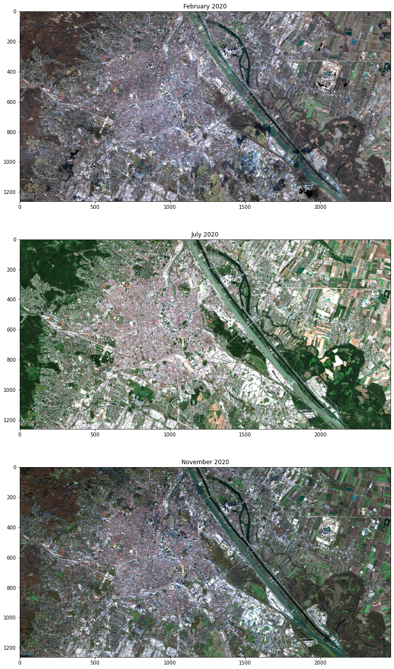

  nodata :

  -9999

plt.figure(figsize=(24,24))

plt.subplot(3,1,1)
output = output_s2.isel(t=0)
plt.title("February 2020")
plt.imshow(tone_mapping(output.B04,output.B03,output.B02), cmap='brg')

plt.subplot(3,1,2)
output = output_s2.isel(t=5)
plt.title("July 2020")
plt.imshow(tone_mapping(output.B04,output.B03,output.B02), cmap='brg')

plt.subplot(3,1,3)
output = output_s2.isel(t=9)
plt.title("November 2020")
plt.imshow(tone_mapping(output.B04,output.B03,output.B02), cmap='brg')

<matplotlib.image.AxesImage at 0x7f16e14e84c0>