Peak-Valley detection in Sentinel-2 NDVI

Peak-Valley detection in Sentinel-2 NDVI#

Welcome to this Jupyter Notebook where we will be working with time series data! Our goal is to download a time series data for a meadow and use the peak-valley detection algorithm originally from FuseTS to extract insights from the data. Time series analysis is a powerful tool that allows us to understand patterns and trends in data over time, and we will be leveraging this tool to analyze the data for the meadow. With the help of the FuseTS peak-valley detection algorithm, we will be able to identify the highest and lowest points in the data, allowing us to gain a better understanding of the underlying patterns and trends.

This notebook copies the FuseTS original to avoid dependency issues in the workshop!

Algorithm type: single pixel timeseries analysis

The actual peak-valley algorithm can be found here:

pangeo-data/pangeo-openeo-BiDS-2023

This is the ‘UDF’ entrypoint: pangeo-data/pangeo-openeo-BiDS-2023

Prerequisites

In this notebook we are using openEO to fetch the time series data for the meadow. You can register for a free trial account on the openEO Platform website.

Lets start with importing the different libraries that we need within this notebook.

#the autoreload extension makes it easier to work with code in a separate python file (peakvalley.py)
%load_ext autoreload
%autoreload 2

import os

import matplotlib.pyplot as plt
import numpy as np
import openeo
import rasterio
import xarray
from rasterio.features import geometry_mask


import importlib
import peakvalley
importlib.reload(peakvalley)

np.random.seed(42)

Downloading the S2 time series#

In order to execute the peak valley algorithm, we need to have time series data. Retrieving time series data can be done through various methods, and one such method is using openEO. OpenEO is an API that provides access to a variety of Earth Observation (EO) data and processing services in a standardized and easy-to-use way. By leveraging the power of openEO, we can easily retrieve the time series data for the meadow and use it to analyze the patterns and trends.

More information on the usage of openEO’s Python client can be found on GitHub.

The first step is to connect to an openEO compatible backend.

connection = openeo.connect("openeo.cloud").authenticate_oidc()

Visit https://aai.egi.eu/device?user_code=KSNO-NMYZ 📋 to authenticate.

[-------------------------------------] ❌ Timed out

---------------------------------------------------------------------------
OidcDeviceCodePollTimeout                 Traceback (most recent call last)
Cell In[2], line 1
----> 1 connection = openeo.connect("openeo.cloud").authenticate_oidc()

File ~/micromamba/envs/bids23/lib/python3.11/site-packages/openeo/rest/connection.py:742, in Connection.authenticate_oidc(self, provider_id, client_id, client_secret, store_refresh_token, use_pkce, display, max_poll_time)
    738 _log.info("Trying device code flow.")
    739 authenticator = OidcDeviceAuthenticator(
    740     client_info=client_info, use_pkce=use_pkce, display=display, max_poll_time=max_poll_time
    741 )
--> 742 con = self._authenticate_oidc(
    743     authenticator,
    744     provider_id=provider_id,
    745     store_refresh_token=store_refresh_token,
    746 )
    747 print("Authenticated using device code flow.")
    748 return con

File ~/micromamba/envs/bids23/lib/python3.11/site-packages/openeo/rest/connection.py:472, in Connection._authenticate_oidc(self, authenticator, provider_id, store_refresh_token, fallback_refresh_token_to_store, oidc_auth_renewer)
    460 def _authenticate_oidc(
    461     self,
    462     authenticator: OidcAuthenticator,
   (...)
    467     oidc_auth_renewer: Optional[OidcAuthenticator] = None,
    468 ) -> Connection:
    469     """
    470     Authenticate through OIDC and set up bearer token (based on OIDC access_token) for further requests.
    471     """
--> 472     tokens = authenticator.get_tokens(request_refresh_token=store_refresh_token)
    473     _log.info("Obtained tokens: {t}".format(t=[k for k, v in tokens._asdict().items() if v]))
    474     if store_refresh_token:

File ~/micromamba/envs/bids23/lib/python3.11/site-packages/openeo/rest/auth/oidc.py:911, in OidcDeviceAuthenticator.get_tokens(self, request_refresh_token)
    908         next_poll = elapsed() + poll_interval
    910 poll_ui.show_progress(status="Timed out")
--> 911 raise OidcDeviceCodePollTimeout(f"Timeout ({self._max_poll_time:.1f}s) while polling for access token.")

OidcDeviceCodePollTimeout: Timeout (300.0s) while polling for access token.

Next we define the area of interest, in this case an extent, for which we would like to fetch time series data.

# set download extent
minx, miny, maxx, maxy = (
    15.179421073198585,
    45.80924633589998,
    15.185336903822831,
    45.81302555710934,
)
spat_ext = dict(west=minx, east=maxx, north=maxy, south=miny, crs=4326)
temp_ext = ["2022-01-01", "2022-12-31"]

We will create an openEO process to calculate the NDVI time series for our area of interest. We’ll begin by using the SENTINEL2_L2A_SENTINELHUB collection, and apply a cloud masking algorithm to remove any interfering clouds before calculating the NDVI values.

# define openEO pipeline
s2 = connection.load_collection(
    "SENTINEL2_L2A",
    spatial_extent=spat_ext,
    temporal_extent=temp_ext,
    bands=["B04", "B08", "SCL"],
    max_cloud_cover=80
)
s2 = s2.process("mask_scl_dilation", data=s2, scl_band_name="SCL")
ndvi_cube = s2.ndvi(red="B04", nir="B08")

/home/driesj/python/openeo-python-client/openeo/rest/connection.py:1171: UserWarning: SENTINEL2_L2A property filtering with properties that are undefined in the collection metadata (summaries): eo:cloud_cover.
  return DataCube.load_collection(

Now that we have calculated the NDVI time series for our area of interest, we can request openEO to download the result to our local storage. This will allow us to access the file and use it for further analysis in this notebook. However, if we have already downloaded the file, we can use the existing time series to continue our analysis without the need for a new download.

%%time
if not os.path.exists("../data/s2_meadow.nc"):
    #job = ndvi_cube.execute_batch("../data/s2_meadow.nc", title=f"FuseTS - Peak Valley - Time Series")
    ndvi_cube.download("../data/s2_meadow.nc")

CPU times: user 514 µs, sys: 100 µs, total: 614 µs
Wall time: 906 µs

ndvi=ds['var']

#download if you already have a job result
#connection.job("vito-j-2311057a8fdb4d7d89d944c693fb2d40").download_result("peakvalley.nc")

PosixPath('peakvalley.nc')

#or create and run a new job
peakvalley.peakvalley(ndvi_cube, drop_thr=0.15, rec_r=1.0, slope_thr=-0.007).execute_batch("peakvalley.nc")

00:00 Job 'vito-j-2311057a8fdb4d7d89d944c693fb2d40': send 'start'
00:18 Job 'vito-j-2311057a8fdb4d7d89d944c693fb2d40': queued (progress N/A)
00:23 Job 'vito-j-2311057a8fdb4d7d89d944c693fb2d40': queued (progress N/A)
00:30 Job 'vito-j-2311057a8fdb4d7d89d944c693fb2d40': queued (progress N/A)
00:38 Job 'vito-j-2311057a8fdb4d7d89d944c693fb2d40': queued (progress N/A)
00:49 Job 'vito-j-2311057a8fdb4d7d89d944c693fb2d40': queued (progress N/A)
01:01 Job 'vito-j-2311057a8fdb4d7d89d944c693fb2d40': queued (progress N/A)
01:18 Job 'vito-j-2311057a8fdb4d7d89d944c693fb2d40': queued (progress N/A)

Now that we have calculated the NDVI time series, we can utilize it to execute the peak valley algorithm that is part of the FuseTS algorithm. The peak valley algorithm is a powerful tool that allows us to detect significant changes in the vegetation patterns over time.

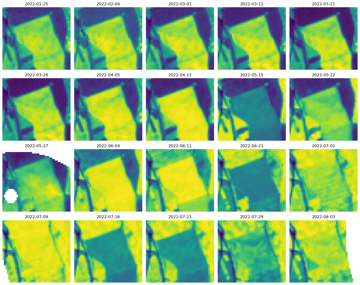
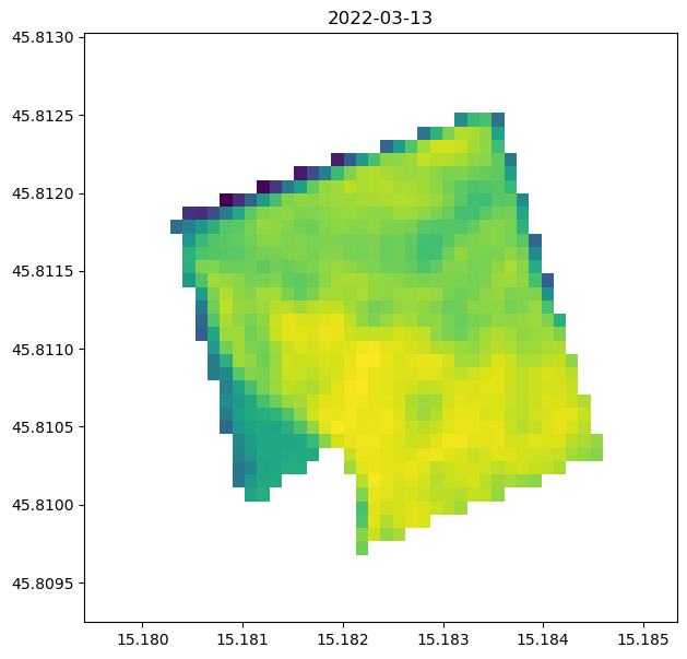
Plot Image Chips Across Time#

# take observations with more 80% of valid data or more
mask = np.count_nonzero(~np.isnan(ndvi), axis=(1, 2)) / np.prod(ndvi[0].shape) > 0.8
ndvi_filtered = ndvi.isel(t=mask)

ncols = 5
nrows = 4
plt.style.use(["default"])
fig, axs = plt.subplots(figsize=(3 * ncols, 3 * nrows), ncols=ncols, nrows=nrows)
fig.patch.set_alpha(1)

for ax, img in zip(axs.flatten(), ndvi_filtered.isel(t=slice(0, -1, 2))):
    ax.imshow(img)
    ax.axis("off")
    ax.set_title(img.t.dt.date.to_numpy())

plt.tight_layout()

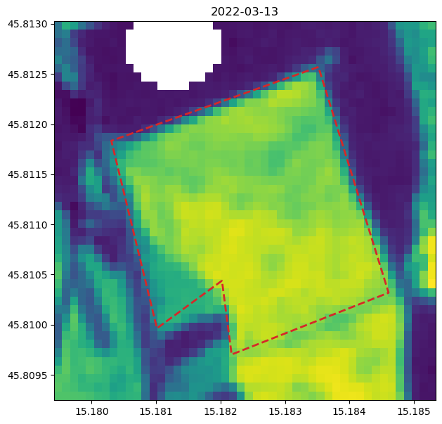
../_images/f6800ecf1e46f6cfc7074d3b2be3befecb790a4937ee6b0d820fe2698c14c952.png

Plot Time Series for Specific Polygon Area#

# define geometry of area-of-interest (AOI)
geometry = {
    "type": "Polygon",
    "coordinates": [
        [
            [15.183519, 45.81257],
            [15.180305, 45.811834],
            [15.181013, 45.809964],
            [15.182022, 45.810439],
            [15.182172, 45.809703],
            [15.184608, 45.810319],
            [15.183519, 45.81257],
        ]
    ],
}

fig, ax = plt.subplots(figsize=(7, 7))

# plot AOI
ax.imshow(ndvi_filtered.isel(t=7), extent=[minx, maxx, miny, maxy])
ax.plot(*np.array(geometry["coordinates"][0]).T, "C3", lw=2, ls="dashed")
ax.set_title(ndvi_filtered.isel(t=7).t.dt.date.to_numpy())
ax.set_aspect("auto")

../_images/0331d9521da4c521f2b94cc00d2516aefba993395de50a34102e8bafd85755c5.png

# define AOI mask
geom_mask = geometry_mask(
    [geometry],
    out_shape=ndvi_filtered[0].shape,
    transform=rasterio.transform.from_bounds(
        *(minx, miny, maxx, maxy),
        width=ndvi_filtered.sizes["x"],
        height=ndvi_filtered.sizes["y"],
    ),
    invert=True,
)
geom_mask = xarray.DataArray(geom_mask, dims=("y", "x"))

# filter to AOI
ndvi_masked = ndvi_filtered.where(geom_mask == True)

fig, ax = plt.subplots(figsize=(7, 7))

# plot result
ax.imshow(ndvi_masked.isel(t=7), extent=[minx, maxx, miny, maxy])
ax.set_title(ndvi_masked.isel(t=7).t.dt.date.to_numpy())
ax.set_aspect("auto")

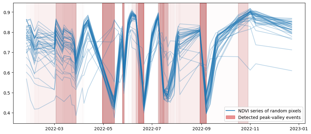
../_images/56e4e632833b39b356a94a60ff340bf55ee30e713e54e05821d6e6ed72576ad1.png

We plot the result two times: once the local computation and then the openEO result. Plots should be the same!

# sample random pixels
valid_x, valid_y = np.where(geom_mask)
rand_x = np.random.choice(valid_x, 50)
rand_y = np.random.choice(valid_y, 50)

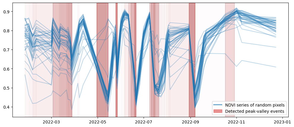
def plot_peak_valley(pv):



    fig, ax = plt.subplots(figsize=(12, 5))

    for idx, idy in zip(rand_x, rand_y):
        # filter potential nan values
        ts = ndvi_masked.isel(x=idx, y=idy)
        ts = ts[~np.isnan(ts)]

        # extract peak-valley info
        data = pv.isel(x=idx, y=idy)
        pairs = np.transpose([np.where(data == 1)[0], np.where(data == -1)[0]])

        # plot time series
        ax.plot(ts.t, ts, "C0", alpha=0.3)

        if len(pairs) > 0:
            for pair in pairs:
                # plot peak-valley span
                ax.axvspan(*data[pair].t.to_numpy(), color="C3", alpha=0.01)

    # add legends
    ax.plot([], [], "C0", label="NDVI series of random pixels")
    ax.axvspan(None, None, color="C3", alpha=0.5, label="Detected peak-valley events")
    ax.legend()
plot_peak_valley(pv_result)
plot_peak_valley(pv_result_openeo['var'])

../_images/6f3b1badf2ea1dc20d6d3ae03fbc877ea1f854700a8292bac770292b1835070b.png

../_images/404fd55214a41a5f87d63aad2151cf5542fb23ca1c2c8654413d82e9514b2e6e.png

Peak-Valley detection in Sentinel-2 NDVI

Contents

Peak-Valley detection in Sentinel-2 NDVI#

Downloading the S2 time series#

Plot Image Chips Across Time#

Plot Time Series for Specific Polygon Area#